Intermediate SSM Analysis • circumplex

library(circumplex)

1. Generalizing the basic analyses

Generalizing to multiple means

We’ve already seen how adding the measures argument can change ssm_analyze() from analyzing means to analyzing correlations. Similarly, we can change it from analyzing all observations as a single group to analyzing subgroups separately. This is done using the grouping argument. This argument needs to contain a single variable (name or column number) that specifies each observation’s group. For instance, the Gender variable in the jz2017 dataset is a factor with two levels: Female and Male. To analyze each gender separately, we need to add the grouping = "Gender" argument to the function call.

data("jz2017")
results <- ssm_analyze(
  data = jz2017, 
  scales = PANO(), 
  angles = octants(), 
  grouping = "Gender"
)
summary(results)
#> 
#> Statistical Basis:    Mean Scores 
#> Bootstrap Resamples:  2000 
#> Confidence Level:     0.95 
#> Listwise Deletion:    TRUE 
#> Scale Displacements:  90 135 180 225 270 315 360 45 
#> 
#> 
#> # Profile [Female]:
#> 
#>                Estimate   Lower CI   Upper CI
#> Elevation         0.946      0.907      0.984
#> X-Value           0.459      0.422      0.498
#> Y-Value          -0.310     -0.357     -0.266
#> Amplitude         0.554      0.511      0.600
#> Displacement    325.963    321.834    329.805
#> Model Fit         0.889                      
#> 
#> 
#> # Profile [Male]:
#> 
#>                Estimate   Lower CI   Upper CI
#> Elevation         0.884      0.839      0.928
#> X-Value           0.227      0.191      0.262
#> Y-Value          -0.186     -0.225     -0.147
#> Amplitude         0.294      0.256      0.330
#> Displacement    320.685    313.386    327.985
#> Model Fit         0.824

Note that the output of summary() looks the same as previous mean-based analyses except that there are now two Profile blocks: one for Female and one for Male. A similar modification will occur if we generate a table and figure.

ssm_table(results)

Mean-based Structural Summary Statistics with 95% CIs
Profile	Elevation	X.Value	Y.Value	Amplitude	Displacement	Fit
Female	0.95 (0.91, 0.98)	0.46 (0.42, 0.50)	-0.31 (-0.36, -0.27)	0.55 (0.51, 0.60)	326.0 (321.8, 329.8)	0.889
Male	0.88 (0.84, 0.93)	0.23 (0.19, 0.26)	-0.19 (-0.23, -0.15)	0.29 (0.26, 0.33)	320.7 (313.4, 328.0)	0.824

ssm_plot_circle(results)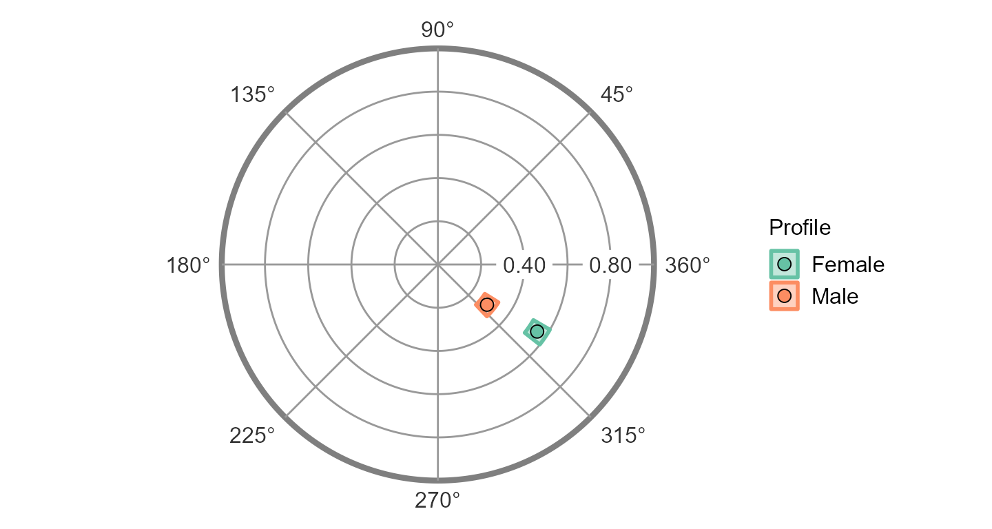

ssm_plot_curve(results)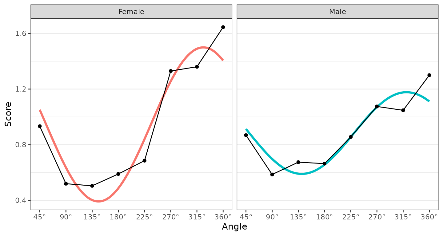

Any number of groups can be analyzed in this way, and the output will contain additional profile blocks, the table will contain additional rows, and the figures will contain additional points or curves. The grouping variable just needs to contain more than one level (i.e., unique value).

Generalizing to multiple measures

Similarly, we can analyze multiple external measures in a single function call by providing a vector of variables to the measures argument instead of a single variable. This can be done by wrapping the variable names or column numbers with the c() or, if they are adjacent columns, with the column numbers and the : shortcut. The package functions were written to analyze all measures and groups within a single bootstrapping, so adding additional measures and groups should still be fast.

results2 <- ssm_analyze(
  data = jz2017, 
  scales = PANO(), 
  angles = octants(),
  measures = c("NARPD", "ASPD")
)
summary(results2)
#> 
#> Statistical Basis:    Correlation Scores 
#> Bootstrap Resamples:  2000 
#> Confidence Level:     0.95 
#> Listwise Deletion:    TRUE 
#> Scale Displacements:  90 135 180 225 270 315 360 45 
#> 
#> 
#> # Profile [NARPD]:
#> 
#>                Estimate   Lower CI   Upper CI
#> Elevation         0.202      0.168      0.236
#> X-Value          -0.062     -0.095     -0.026
#> Y-Value           0.179      0.145      0.214
#> Amplitude         0.189      0.155      0.225
#> Displacement    108.967     98.853    118.517
#> Model Fit         0.957                      
#> 
#> 
#> # Profile [ASPD]:
#> 
#>                Estimate   Lower CI   Upper CI
#> Elevation         0.124      0.090      0.157
#> X-Value          -0.099     -0.134     -0.063
#> Y-Value           0.203      0.168      0.240
#> Amplitude         0.226      0.188      0.265
#> Displacement    115.927    107.250    124.516
#> Model Fit         0.964

ssm_table(results2)

Correlation-based Structural Summary Statistics with 95% CIs
Profile	Elevation	X.Value	Y.Value	Amplitude	Displacement	Fit
NARPD	0.20 (0.17, 0.24)	-0.06 (-0.09, -0.03)	0.18 (0.14, 0.21)	0.19 (0.15, 0.22)	109.0 (98.9, 118.5)	0.957
ASPD	0.12 (0.09, 0.16)	-0.10 (-0.13, -0.06)	0.20 (0.17, 0.24)	0.23 (0.19, 0.27)	115.9 (107.2, 124.5)	0.964

ssm_plot_circle(results2)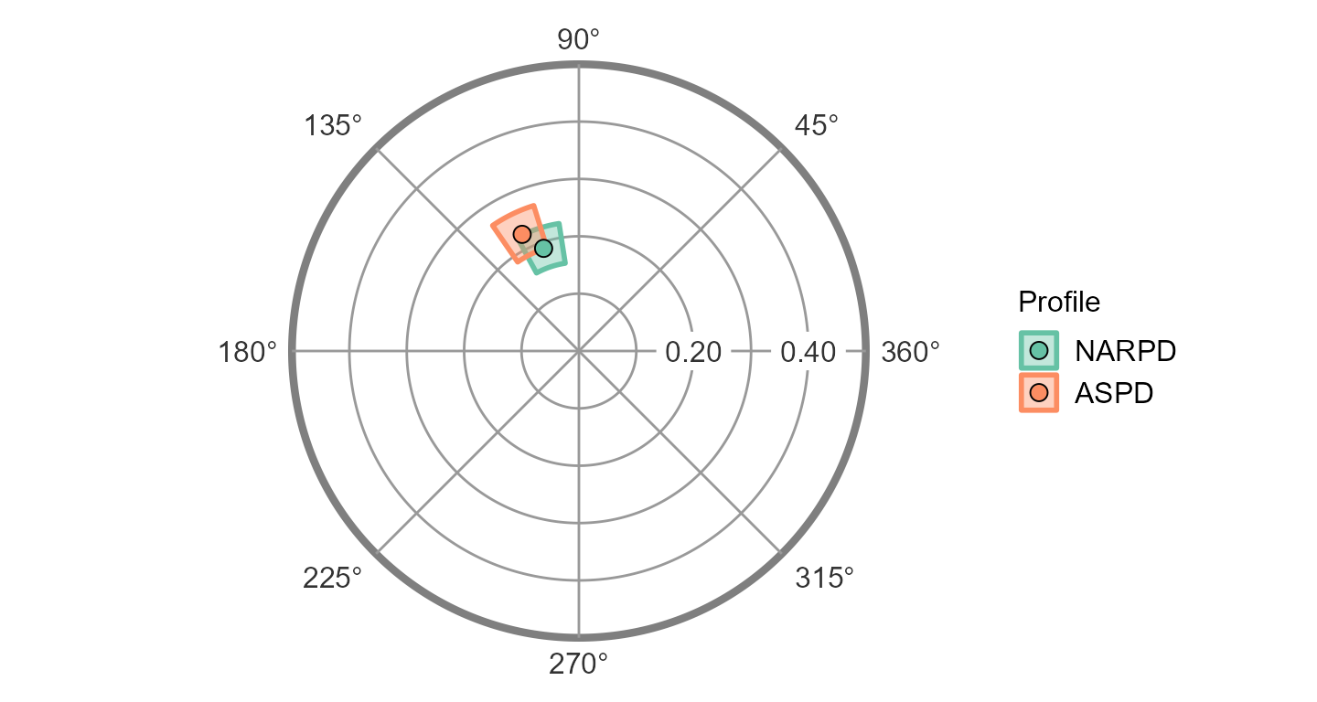

ssm_plot_curve(results2)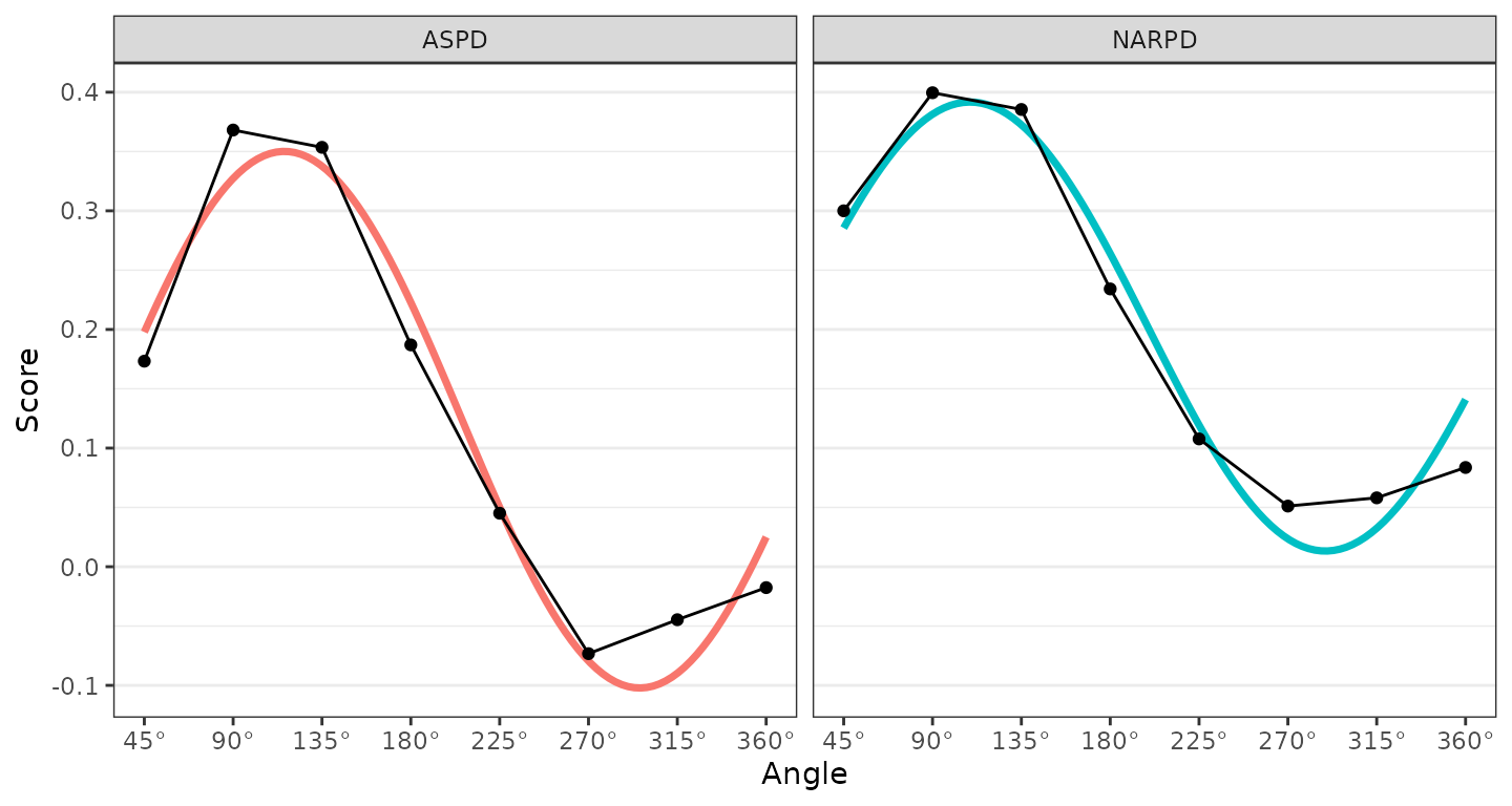

Generalizing to multiple groups and multiple measures

Finally, it is possible to analyze multiple measures within multiple groups. As you might expect, this requires providing both the measures and grouping arguments to the same function call. Again, any number of measures and groups is possible. The profiles in such an analysis will be named “Measure: Group” as below.

results3 <- ssm_analyze(
  data = jz2017, 
  scales = PANO(), 
  angles = octants(), 
  grouping = "Gender", 
  measures = 10:12)
summary(results3)
#> 
#> Statistical Basis:    Correlation Scores 
#> Bootstrap Resamples:  2000 
#> Confidence Level:     0.95 
#> Listwise Deletion:    TRUE 
#> Scale Displacements:  90 135 180 225 270 315 360 45 
#> 
#> 
#> # Profile [PARPD: Female]:
#> 
#>                Estimate   Lower CI   Upper CI
#> Elevation         0.262      0.220      0.305
#> X-Value          -0.146     -0.192     -0.100
#> Y-Value           0.120      0.070      0.171
#> Amplitude         0.189      0.137      0.243
#> Displacement    140.524    126.580    155.129
#> Model Fit         0.870                      
#> 
#> 
#> # Profile [SCZPD: Female]:
#> 
#>                Estimate   Lower CI   Upper CI
#> Elevation         0.177      0.130      0.218
#> X-Value          -0.230     -0.285     -0.173
#> Y-Value          -0.047     -0.103      0.006
#> Amplitude         0.235      0.185      0.288
#> Displacement    191.613    178.684    208.113
#> Model Fit         0.845                      
#> 
#> 
#> # Profile [SZTPD: Female]:
#> 
#>                Estimate   Lower CI   Upper CI
#> Elevation         0.237      0.194      0.280
#> X-Value          -0.130     -0.175     -0.087
#> Y-Value           0.016     -0.037      0.069
#> Amplitude         0.131      0.090      0.180
#> Displacement    172.870    151.247    198.040
#> Model Fit         0.812                      
#> 
#> 
#> # Profile [PARPD: Male]:
#> 
#>                Estimate   Lower CI   Upper CI
#> Elevation         0.243      0.193      0.288
#> X-Value          -0.035     -0.080      0.015
#> Y-Value           0.114      0.066      0.165
#> Amplitude         0.120      0.075      0.171
#> Displacement    106.881     82.677    129.996
#> Model Fit         0.648                      
#> 
#> 
#> # Profile [SCZPD: Male]:
#> 
#>                Estimate   Lower CI   Upper CI
#> Elevation         0.204      0.145      0.260
#> X-Value          -0.178     -0.220     -0.136
#> Y-Value          -0.017     -0.071      0.039
#> Amplitude         0.179      0.139      0.222
#> Displacement    185.351    167.551    203.091
#> Model Fit         0.917                      
#> 
#> 
#> # Profile [SZTPD: Male]:
#> 
#>                Estimate   Lower CI   Upper CI
#> Elevation         0.240      0.186      0.293
#> X-Value          -0.037     -0.084      0.011
#> Y-Value           0.029     -0.018      0.079
#> Amplitude         0.047      0.013      0.101
#> Displacement    142.345     68.178    218.702
#> Model Fit         0.424

ssm_table(results3)

Correlation-based Structural Summary Statistics with 95% CIs
Profile	Elevation	X.Value	Y.Value	Amplitude	Displacement	Fit
PARPD: Female	0.26 (0.22, 0.30)	-0.15 (-0.19, -0.10)	0.12 (0.07, 0.17)	0.19 (0.14, 0.24)	140.5 (126.6, 155.1)	0.870
SCZPD: Female	0.18 (0.13, 0.22)	-0.23 (-0.29, -0.17)	-0.05 (-0.10, 0.01)	0.23 (0.19, 0.29)	191.6 (178.7, 208.1)	0.845
SZTPD: Female	0.24 (0.19, 0.28)	-0.13 (-0.18, -0.09)	0.02 (-0.04, 0.07)	0.13 (0.09, 0.18)	172.9 (151.2, 198.0)	0.812
PARPD: Male	0.24 (0.19, 0.29)	-0.03 (-0.08, 0.01)	0.11 (0.07, 0.17)	0.12 (0.07, 0.17)	106.9 (82.7, 130.0)	0.648
SCZPD: Male	0.20 (0.15, 0.26)	-0.18 (-0.22, -0.14)	-0.02 (-0.07, 0.04)	0.18 (0.14, 0.22)	185.4 (167.6, 203.1)	0.917
SZTPD: Male	0.24 (0.19, 0.29)	-0.04 (-0.08, 0.01)	0.03 (-0.02, 0.08)	0.05 (0.01, 0.10)	142.3 (68.2, 218.7)	0.424

ssm_plot_circle(results3)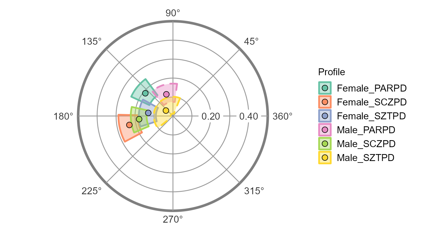

Note that the borders for the “PARDPD: Male” and “SZTPD: Male” blocks are dashed instead of solid. This indicates that these profiles have low fit (i.e., $R^2<.7$ ). We could alternatively hide these such profiles by adding lowfit = FALSE as below (noting that the color guide may change as profiles are dropped).

ssm_plot_circle(results3, drop_lowfit = TRUE)

ssm_plot_curve(results3)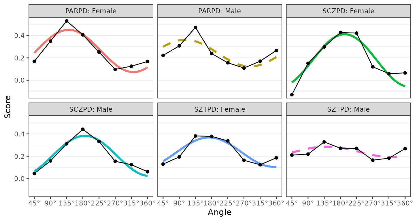

ssm_plot_curve(results3, drop_lowfit = TRUE)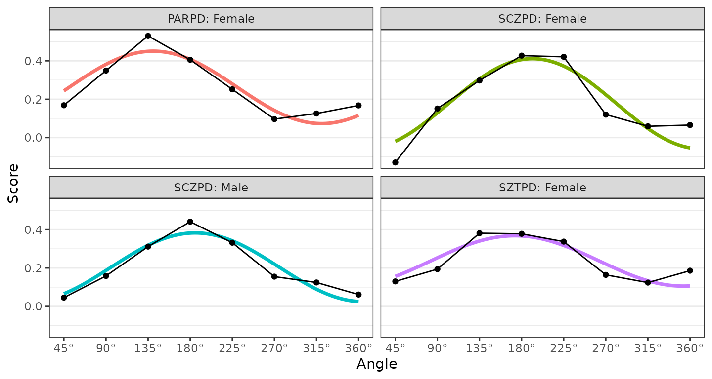

2. Contrast analyses

The final argument to master in this vignette is contrast, which allows us to compare two groups or measures. Setting this argument to TRUE will first generate scores for each group (or measure), then estimate SSM parameters for these scores, and finally calculate the difference between the parameters. To keep the code simpler and to discourage “fishing expeditions,” only two groups or measures can be compared at a time.

Contrasts between groups’ means

To compare the mean profiles for females and males, we can start with the same syntax we had before and then add a contrast argument.

results4 <- ssm_analyze(
  data = jz2017, 
  scales = PANO(), 
  angles = octants(), 
  grouping = "Gender", 
  contrast = TRUE
)
summary(results4)
#> 
#> Statistical Basis:    Mean Scores 
#> Bootstrap Resamples:  2000 
#> Confidence Level:     0.95 
#> Listwise Deletion:    TRUE 
#> Scale Displacements:  90 135 180 225 270 315 360 45 
#> 
#> 
#> # Profile [Female]:
#> 
#>                Estimate   Lower CI   Upper CI
#> Elevation         0.946      0.908      0.984
#> X-Value           0.459      0.419      0.498
#> Y-Value          -0.310     -0.353     -0.269
#> Amplitude         0.554      0.510      0.599
#> Displacement    325.963    322.251    329.698
#> Model Fit         0.889                      
#> 
#> 
#> # Profile [Male]:
#> 
#>                Estimate   Lower CI   Upper CI
#> Elevation         0.884      0.841      0.925
#> X-Value           0.227      0.191      0.261
#> Y-Value          -0.186     -0.225     -0.148
#> Amplitude         0.294      0.256      0.331
#> Displacement    320.685    313.293    327.938
#> Model Fit         0.824                      
#> 
#> 
#> # Contrast [Male - Female]:
#> 
#>                  Estimate   Lower CI   Upper CI
#> Δ Elevation        -0.062     -0.119     -0.004
#> Δ X-Value          -0.232     -0.285     -0.181
#> Δ Y-Value           0.124      0.066      0.183
#> Δ Amplitude        -0.261     -0.318     -0.203
#> Δ Displacement     -5.278    -13.627      2.178
#> Δ Model Fit        -0.066

Note that we have the profile blocks for each group as well as a contrast block. The contrast is made by subtracting the first level of the grouping variable from the second level (e.g., Male - Female). This provides an indication of the direction of the contrast. We can again generate a table and figure to display the results.

ssm_table(results4)

Mean-based Structural Summary Statistic Contrasts with 95% CIs
Contrast	Elevation	X.Value	Y.Value	Amplitude	Displacement	Fit
Female	0.95 (0.91, 0.98)	0.46 (0.42, 0.50)	-0.31 (-0.35, -0.27)	0.55 (0.51, 0.60)	326.0 (322.3, 329.7)	0.889
Male	0.88 (0.84, 0.93)	0.23 (0.19, 0.26)	-0.19 (-0.22, -0.15)	0.29 (0.26, 0.33)	320.7 (313.3, 327.9)	0.824
Male - Female	-0.06 (-0.12, -0.00)	-0.23 (-0.29, -0.18)	0.12 (0.07, 0.18)	-0.26 (-0.32, -0.20)	-5.3 (-13.6, 2.2)	-0.066

ssm_plot_contrast(results4)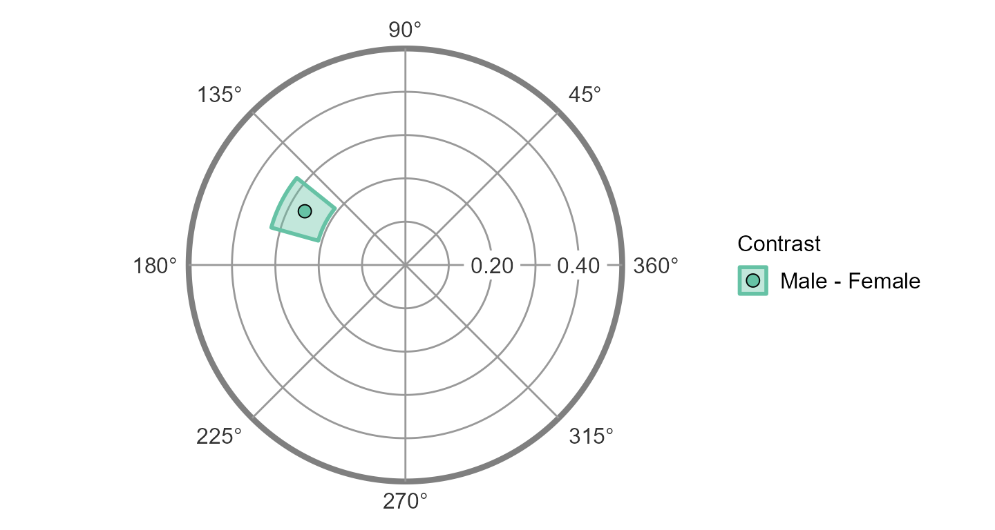

Contrasts between measures in a group

Comparing measures in a group is very similar. Again, all we need to do is add the contrast argument to the function call containing measures. Here we will use a parameter contrast to see what they look like.

results5 <- ssm_analyze(
  data = jz2017, 
  scales = PANO(), 
  angles = octants(), 
  measures = c("NARPD", "ASPD"),
  contrast = TRUE
)
summary(results5)
#> 
#> Statistical Basis:    Correlation Scores 
#> Bootstrap Resamples:  2000 
#> Confidence Level:     0.95 
#> Listwise Deletion:    TRUE 
#> Scale Displacements:  90 135 180 225 270 315 360 45 
#> 
#> 
#> # Profile [NARPD]:
#> 
#>                Estimate   Lower CI   Upper CI
#> Elevation         0.202      0.169      0.233
#> X-Value          -0.062     -0.097     -0.029
#> Y-Value           0.179      0.144      0.212
#> Amplitude         0.189      0.154      0.226
#> Displacement    108.967     99.122    118.902
#> Model Fit         0.957                      
#> 
#> 
#> # Profile [ASPD]:
#> 
#>                Estimate   Lower CI   Upper CI
#> Elevation         0.124      0.091      0.159
#> X-Value          -0.099     -0.135     -0.065
#> Y-Value           0.203      0.166      0.237
#> Amplitude         0.226      0.190      0.265
#> Displacement    115.927    107.571    124.311
#> Model Fit         0.964                      
#> 
#> 
#> # Contrast [ASPD - NARPD]:
#> 
#>                  Estimate   Lower CI   Upper CI
#> Δ Elevation        -0.079     -0.114     -0.043
#> Δ X-Value          -0.037     -0.074      0.002
#> Δ Y-Value           0.024     -0.014      0.061
#> Δ Amplitude         0.037     -0.002      0.075
#> Δ Displacement      6.960     -3.391     17.383
#> Δ Model Fit         0.007

ssm_table(results5)

Correlation-based Structural Summary Statistic Contrasts with 95% CIs
Contrast	Elevation	X.Value	Y.Value	Amplitude	Displacement	Fit
NARPD	0.20 (0.17, 0.23)	-0.06 (-0.10, -0.03)	0.18 (0.14, 0.21)	0.19 (0.15, 0.23)	109.0 (99.1, 118.9)	0.957
ASPD	0.12 (0.09, 0.16)	-0.10 (-0.13, -0.06)	0.20 (0.17, 0.24)	0.23 (0.19, 0.26)	115.9 (107.6, 124.3)	0.964
ASPD - NARPD	-0.08 (-0.11, -0.04)	-0.04 (-0.07, 0.00)	0.02 (-0.01, 0.06)	0.04 (-0.00, 0.08)	7.0 (-3.4, 17.4)	0.007

ssm_plot_contrast(results5)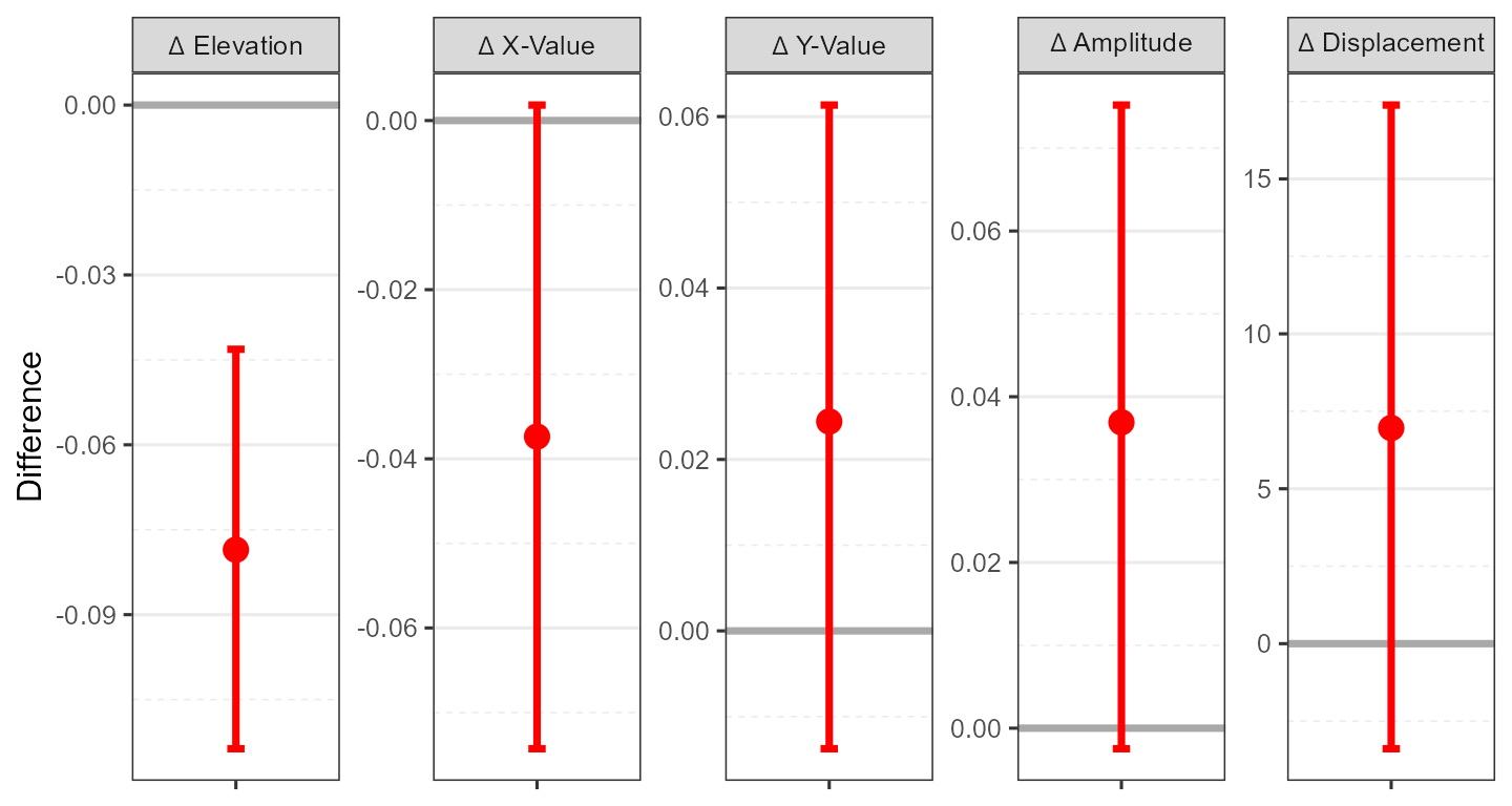

Here, instead of a circle plot, we see a contrast plot showing the difference between the two measures’ SSM parameters and their 95% confidence intervals. Because the confidence interval for the elevation parameter does not include zero, this parameter is significantly different between the measures.

Contrasts between groups’ correlations

Finally, we might want to compare a single measure’s profiles in two different groups. To do so, we need to specify the measures, the grouping variable, and the type of contrast. In this case, we need to ensure that we are providing only a single measure and a grouping variable with just two levels (as again only two things can be contrasted at a time). Note that the contrast name in this case will take the form of “Measure: Group2 - Group1”.

results6 <- ssm_analyze(
  data = jz2017, 
  scales = PANO(), 
  angles = octants(), 
  measures = "BORPD", 
  grouping = "Gender", 
  contrast = TRUE
)
summary(results6)
#> 
#> Statistical Basis:    Correlation Scores 
#> Bootstrap Resamples:  2000 
#> Confidence Level:     0.95 
#> Listwise Deletion:    TRUE 
#> Scale Displacements:  90 135 180 225 270 315 360 45 
#> 
#> 
#> # Profile [BORPD: Female]:
#> 
#>                Estimate   Lower CI   Upper CI
#> Elevation         0.251      0.206      0.293
#> X-Value          -0.068     -0.114     -0.021
#> Y-Value           0.126      0.064      0.184
#> Amplitude         0.143      0.084      0.203
#> Displacement    118.247     99.973    138.946
#> Model Fit         0.947                      
#> 
#> 
#> # Profile [BORPD: Male]:
#> 
#>                Estimate   Lower CI   Upper CI
#> Elevation         0.320      0.267      0.370
#> X-Value           0.012     -0.034      0.058
#> Y-Value           0.054      0.004      0.106
#> Amplitude         0.055      0.016      0.109
#> Displacement     77.367     12.983    133.991
#> Model Fit         0.500                      
#> 
#> 
#> # Contrast [BORPD: Male - Female]:
#> 
#>                  Estimate   Lower CI   Upper CI
#> Δ Elevation         0.069      0.000      0.136
#> Δ X-Value           0.080      0.017      0.146
#> Δ Y-Value          -0.072     -0.152      0.010
#> Δ Amplitude        -0.088     -0.160     -0.003
#> Δ Displacement    -40.880   -105.533     19.259
#> Δ Model Fit        -0.447

ssm_table(results6)

Correlation-based Structural Summary Statistic Contrasts with 95% CIs
Contrast	Elevation	X.Value	Y.Value	Amplitude	Displacement	Fit
BORPD: Female	0.25 (0.21, 0.29)	-0.07 (-0.11, -0.02)	0.13 (0.06, 0.18)	0.14 (0.08, 0.20)	118.2 (100.0, 138.9)	0.947
BORPD: Male	0.32 (0.27, 0.37)	0.01 (-0.03, 0.06)	0.05 (0.00, 0.11)	0.06 (0.02, 0.11)	77.4 (13.0, 134.0)	0.500
BORPD: Male - Female	0.07 (0.00, 0.14)	0.08 (0.02, 0.15)	-0.07 (-0.15, 0.01)	-0.09 (-0.16, -0.00)	-40.9 (-105.5, 19.3)	-0.447

ssm_plot_contrast(results6)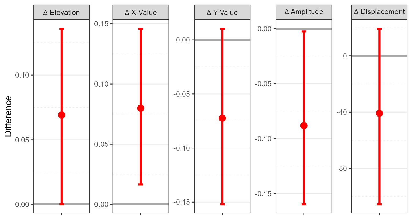

3. Taxonomy of analysis types

Although all SSM analyses are based on the idea of decomposing circumplex scores into the parameters of a cosine curve, there are actually many different ways to implement it. Each of these implementations allows different questions to be explored. In the table below, a list of the SSM analysis types that are currently implemented in the circumplex package is provided. This table also provides the specific combination of arguments needed to implement each analysis using the ssm_analyze() function. Specifying which analysis to run is simply a matter of providing the correct arguments to the function; this allows a single function to essentially do the work of seven and makes for a more intuitive user experience.

	Arguments Needed
Usage	measures	grouping	contrast
Examine overall mean profile	FALSE	FALSE	FALSE
Examine groups’ mean profiles	FALSE	TRUE	FALSE
Compare groups’ mean profiles	FALSE	TRUE	TRUE
Examine variables’ correlation profiles	TRUE	FALSE	FALSE
Compare variables’ correlation profiles	TRUE	FALSE	TRUE
Examine groups’ correlation profiles	TRUE	TRUE	FALSE
Compare groups’ correlation profiles	TRUE	TRUE	TRUE

The three main questions to ask when conducting a new SSM analysis are:

Do we want to project non-circumplex measures into the circumplex space? If yes, we must specify one or more measures, and the scores that get modeled using SSM will be the correlations between the circumplex scales and these measures. If no, we must omit the measures argument, and the scores that get modeled using SSM will be the mean scores on the circumplex scales.
Do we want to perform analyses separately for groups within the dataset? If yes, we must specify a grouping variable, and the output will contain results for each group (i.e., unique value of this variable). If no, we must omit the grouping argument, and a single set of results for all data will be output.
Do we want to contrast/compare two sets of results? If yes, we must specify contrast as TRUE and ensure that we are only requesting two sets of results (i.e., two groups or two measures). If no, we must omit the contrast argument or set it to FALSE, and the results themselves will be output, rather than their contrast.

4. Working with SSM tables

Basic customizations of tables

Additional arguments to the ssm_table() function can be explored using the ?ssm_table command. Two useful options are the drop_xy argument, which shows or hides the x-value and y-value columns, and the caption argument which allows a custom string to be printed above the table. Note as well that the return object of this function is just a data frame, which can be easily edited to add, change, or remove text. To change the formatting of the table, see the htmlTable or kableExtra packages.

5. Working with SSM figures

Exporting figures as files

All SSM plots are created using the ggplot2 package, which is incredibly flexible and powerful. It also offers the ggsave() function to export figures to external files of various types. See the documentation for this function (?ggsave) to learn more, but some useful arguments are filename, plot, width, height, and units. We can save the figure as a raster image file (e.g., “png”, “jpeg”, “tiff”), a vector image file (e.g., “svg”), or a portable document (e.g., “pdf” or “tex”). We can also control the exact width and height of the image in different units (i.e., “in”, “cm”, or “mm”). Because the underlying graphics are vectorized in R, they can be easily scaled to any size without loss of quality and used in manuscripts, presentations, or posters.

ssm_plot(results6)
ggsave("bordpd_gender.png", width = 7.5, height = 4, units = "in")

Wrap-up

In this vignette, we learned how to generalize the SSM analyses to multiple groups and measures, how to conduct contrast analyses, how to make basic customizations to tables and figures, and how to export tables and figures to external files. In the next vignette, “Advanced Circumplex Visualization,” we will learn more advanced customization options for the SSM figures and other circumplex visualizations. (Note that the next vignette is still in progress.)

References

Gurtman, M. B. (1992). Construct validity of interpersonal personality measures: The interpersonal circumplex as a nomological net. Journal of Personality and Social Psychology, 63(1), 105–118.
Gurtman, M. B., & Pincus, A. L. (2003). The circumplex model: Methods and research applications. In J. A. Schinka & W. F. Velicer (Eds.), Handbook of psychology. Volume 2: Research methods in psychology (pp. 407–428). Hoboken, NJ: John Wiley & Sons, Inc.
Wright, A. G. C., Pincus, A. L., Conroy, D. E., & Hilsenroth, M. J. (2009). Integrating methods to optimize circumplex description and comparison of groups. Journal of Personality Assessment, 91(4), 311–322.
Zimmermann, J., & Wright, A. G. C. (2017). Beyond description in interpersonal construct validation: Methodological advances in the circumplex Structural Summary Approach. Assessment, 24(1), 3–23.