Bayesian SSM Analysis • circumplex

library(circumplex)

1. Why a Bayesian SSM?

The Structural Summary Method (SSM) describes a circumplex profile with an elevation $e$ , an amplitude $a$ , and a displacement $d$ . The package’s ssm_analyze() estimates these with bootstrap or Monte Carlo confidence intervals. A Bayesian alternative is attractive when you want prior information, hierarchical structure (e.g., partial pooling across persons or groups), or full posterior distributions for derived quantities.

The division of labor is deliberate: a general-purpose Bayesian package such as brms fits the model, and ssm_draws() converts the resulting posterior draws into SSM parameter draws and summarizes them with the same circular-statistics machinery the rest of the package uses. Displacement is an angle, so its posterior needs circular treatment — an interval straddling the 0°/360° boundary must wrap rather than invert — and ssm_draws() handles that by construction.

2. The cosine model as a linear regression

The SSM’s cosine model for a profile of scores $S_j$ observed at scale angles $\theta_j$ is

$S_j = e + a \cos(\theta_j - d).$

Expanding the cosine of a difference gives

$S_j = e + \underbrace{a \cos d}_{x} \cos \theta_j + \underbrace{a \sin d}_{y} \sin \theta_j,$

a linear regression of the scores on $\cos \theta_j$ and $\sin \theta_j$ . The intercept is the elevation $e$ , the cosine coefficient is $x$ , and the sine coefficient is $y$ . The structural parameters are recovered by

$a = \sqrt{x^2 + y^2}, \qquad d = \operatorname{atan2}(y,\, x),$

with the displacement wrapped into $[0°, 360°)$ .

Note the argument order: atan2(y, x) takes the sine coefficient first. Swapping the arguments is a classic silent error — it returns a valid-looking angle that is wrong for almost every profile. The following check pins the convention with a profile whose displacement is known to be 90°, where the swapped call would instead return 0°:

# Truth: e = 1, a = 2, d = 90 degrees
theta <- as.numeric(octants()) * pi / 180
scores <- 1 + 2 * cos(theta - pi / 2)
fit <- lm(scores ~ cos(theta) + sin(theta))
x_hat <- coef(fit)[["cos(theta)"]]
y_hat <- coef(fit)[["sin(theta)"]]
d_hat <- atan2(y_hat, x_hat) * 180 / pi
round(c(x = x_hat, y = y_hat, d = d_hat), 6)
#>  x  y  d 
#>  0  2 90
stopifnot(isTRUE(all.equal(d_hat, 90)))          # atan2(y, x): correct
stopifnot(!isTRUE(all.equal(atan2(x_hat, y_hat) * 180 / pi, 90)))  # swapped

3. Fitting the model with brms

We model raw octant scores from the jz2017 data in long format (one row per person-scale observation), with a random intercept per person to absorb the dependence among a person’s eight scores. The fixed effects (intercept, cosine coefficient, sine coefficient) are then the group-level $(e, x, y)$ . A seeded subsample of 200 persons keeps the example light.

data("jz2017")
set.seed(12345)
sub <- jz2017[sample(nrow(jz2017), 200), ]
scales <- c("PA", "BC", "DE", "FG", "HI", "JK", "LM", "NO")
theta <- as.numeric(octants()) * pi / 180
dat <- data.frame(
  id = rep(seq_len(200), times = length(scales)),
  cos_theta = rep(cos(theta), each = 200),
  sin_theta = rep(sin(theta), each = 200),
  score = unlist(sub[scales], use.names = FALSE)
)
head(dat)
#>   id    cos_theta sin_theta score
#> 1  1 6.123234e-17         1  1.00
#> 2  2 6.123234e-17         1  0.25
#> 3  3 6.123234e-17         1  0.50
#> 4  4 6.123234e-17         1  0.75
#> 5  5 6.123234e-17         1  0.00
#> 6  6 6.123234e-17         1  0.50

Because Bayesian sampling requires a working Stan toolchain, the model below is not re-fitted when this vignette is rebuilt; its posterior draws were generated once by the seeded script data-raw/bayesian_ssm_draws.R and ship with the package. The normal(0, 1) prior on the regression coefficients is a deliberate modeling choice whose consequences for the amplitude we examine in Section 5.

library(brms)
bfit <- brm(
  score ~ cos_theta + sin_theta + (1 | id),
  data = dat,
  prior = set_prior("normal(0, 1)", class = "b"),
  chains = 4, iter = 2000, cores = 4, seed = 12345
)
draws <- as.matrix(bfit,
                   variable = c("b_Intercept", "b_cos_theta", "b_sin_theta"))

4. From posterior draws to SSM summaries

The draws form a matrix with one row per posterior draw and three columns interpreted in column order as $(e, x, y)$ :

draws <- readRDS("bayesian_ssm_draws.rds")
dim(draws)
#> [1] 4000    3
head(round(draws, 3))
#>     variable
#> draw b_Intercept b_cos_theta b_sin_theta
#>    1       0.990       0.315      -0.294
#>    2       0.938       0.382      -0.353
#>    3       0.931       0.356      -0.331
#>    4       0.921       0.339      -0.277
#>    5       0.946       0.382      -0.295
#>    6       0.913       0.355      -0.313

ssm_draws() accepts two draw shapes: three-column parameter draws like these, or profile draws (one column per scale, with angles supplied). A three-column matrix without angles is ambiguous — it could also be profile draws from a three-scale instrument — so the shape must be stated explicitly with type = "parameters":

res <- ssm_draws(draws, type = "parameters")
summary(res)
#> 
#> Statistical Basis:   Posterior Draws 
#> Posterior Draws:  4000 
#> Credible Level:       0.95 
#> Draw Shape:       Parameters 
#> 
#> # Posterior Summary:
#> 
#>                Estimate   Lower CrI   Upper CrI
#> Elevation         0.933       0.868       0.998
#> X-Value           0.352       0.303       0.401
#> Y-Value          -0.319      -0.365      -0.273
#> Amplitude         0.476       0.427       0.522
#> Displacement    317.790     312.274     323.286
#> Model Fit

Each posterior draw of $(x, y)$ was converted to a draw of $(a, d)$ , so the displacement’s credible interval comes from circular quantiles (centered on the circular mean and re-wrapped), never from naive linear quantiles that would misbehave near 0°/360°. Point estimates are posterior medians for the linear parameters — the amplitude posterior is right-skewed, so a mean would overstate it — and the circular mean for displacement. One caveat to keep in mind: these marginal summaries are not jointly coherent. The reported amplitude is the median of the amplitude draws, which is not $\sqrt{x^2 + y^2}$ evaluated at the reported $x$ and $y$ , and the reported displacement is not the direction of the reported $(x, y)$ . Each is the honest marginal summary of its own posterior.

Model fit ( $R^2$ ) is not reported here: parameter draws carry no profile to measure fit against. Feeding ssm_draws() profile draws (shape B) does yield fit draws.

5. The induced prior on amplitude

Independent priors on $x$ and $y$ do not induce a flat prior on the structural parameters. With $x, y \sim \mathrm{Normal}(0, 1)$ , the implied prior on $a = \sqrt{x^2 + y^2}$ is Rayleigh-shaped — its mass is pushed away from $a = 0$ — while the implied prior on $d$ is uniform. A ten-line prior-predictive simulation makes this visible:

x_prior <- rnorm(10000, 0, 1)
y_prior <- rnorm(10000, 0, 1)
a_prior <- sqrt(x_prior^2 + y_prior^2)
ggplot(data.frame(a = a_prior), aes(x = a)) +
  geom_histogram(bins = 60, fill = "grey35") +
  labs(
    x = "Amplitude implied by the priors on x and y",
    y = "Prior draws",
    title = "Rayleigh-shaped induced prior on amplitude"
  ) +
  theme_minimal()

round(c(prior_median = median(a_prior), prior_mass_below_0.1 =
          mean(a_prior < 0.1)), 3)
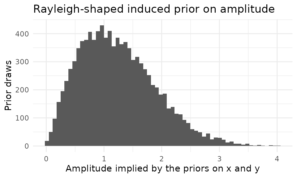
#>         prior_median prior_mass_below_0.1 
#>                1.164                0.005

This is not a defect — it is a modeling choice to be aware of: the prior mildly disfavors exactly-flat profiles. If your application needs prior mass concentrated near $a = 0$ , place priors on $(a, d)$ directly in a custom Stan model instead; its posterior draws can still be summarized here by converting them to $(x, y) = (a \cos d, a \sin d)$ or by passing profile draws.

6. Where to go next

Per-person descriptive SSM parameters (no pooling): ssm_parameters_id() and its summary() method.
Hierarchical pooling across persons or groups is exactly what the brms/Stan route is for — fit the model you need and feed the posterior draws (parameter or profile shape) back through ssm_draws().
Frequentist inference on group profiles and contrasts: ssm_analyze().