SEM-Based SSM Analysis • circumplex

library(circumplex)

The other vignettes model observed circumplex scores: the mean profile of a group, or the profile of correlations between the circumplex scales and an external measure. This vignette introduces a latent counterpart, built on a structural equation model (SEM) of the circumplex scales, and exposed through ssm_sem() and its helpers. It teaches two products — the latent profile of a measure and the invariance-gated latent contrast between groups — how their confidence intervals are constructed, and the assumptions that make them interpretable.

The latent-level Structural Summary Method appears to be new: a search of the SEM–circumplex literature (2019 onward) found related work on the latent structure of circumplex scales (e.g., Wendt et al., 2019) and on inference for disattenuated correlations (Moss, 2026), but no prior work applying the SSM decomposition — elevation, amplitude, displacement, and fit — to a measure’s latent profile with circular-aware intervals. Treat this layer as a research tool whose assumptions you should understand before relying on it.

1. Why a latent SSM?

An observed correlation profile is attenuated by measurement error: because each circumplex scale is imperfectly reliable, the correlations between the scales and an external measure are pulled toward zero, and — because the scales are not equally reliable — pulled toward zero by different amounts. The observed SSM parameters inherit both effects. Amplitude is deflated by the average unreliability, and displacement is rotated by the heterogeneity of reliability around the circle.

The latent SSM estimates the profile the measure would show against the latent circumplex content of the scales — the disattenuated analog of the observed correlation profile (Zimmermann & Wright, 2017, defined the observed version; this is its latent counterpart). It fits a measurement model in which each scale loads on latent factors placed at that scale’s fixed theoretical angle, then reads the measure’s correlations with the common circumplex content and summarizes them with the usual SSM transform.

Two consequences are worth stating up front, because they shape everything below:

The latent profile is model-conditional. Every latent parameter is conditional on the fixed-angle measurement model being an adequate description of the data. A poorly fitting model does not make the latent parameters merely imprecise; it makes them uninterpretable. Global fit is therefore reported alongside every result.
The angles are theoretical claims, not estimates. ssm_sem() never estimates an angle. If an instrument’s real geometry departs from theory, that departure is absorbed into misfit, not into the angles. To examine circumplex geometry — to let the angles be free — use cpm_fit(), which fits Browne’s (1992) circumplex model; that is a different question and a different tool.

2. The measurement model

ssm_sem() builds and fits a lavaan measurement model for you, but it is worth seeing the model it generates. ssm_sem_syntax() returns that model as a string:

scales <- c("PA", "BC", "DE", "FG", "HI", "JK", "LM", "NO")
syntax <- ssm_sem_syntax(scales = scales, angles = octants(), measures = "NARPD")
cat(syntax)
#> # circumplex SSM measurement model (generated by ssm_sem_syntax())
#> # scales: PA, BC, DE, FG, HI, JK, LM, NO
#> # angles (degrees): 90, 135, 180, 225, 270, 315, 360, 45
#> # model tier: scaled
#> 
#> # general factor: free per-scale saturations
#> g =~ NA*PA + a1*PA + a2*BC + a3*DE + a4*FG + a5*HI + a6*JK + a7*LM + a8*NO
#> # circumplex plane: loadings free but with each scale's angle fixed
#> cx =~ NA*PA + lx1*PA + lx2*BC + lx3*DE + lx4*FG + lx5*HI + lx6*JK + lx7*LM + lx8*NO
#> cy =~ NA*PA + ly1*PA + ly2*BC + ly3*DE + ly4*FG + ly5*HI + ly6*JK + ly7*LM + ly8*NO
#> # fixed-angle direction constraints: sin(a)*lx - cos(a)*ly == 0
#> 0 == 1*lx1 - 0*ly1
#> 0 == 0.70710678118654757*lx2 - -0.70710678118654746*ly2
#> 0 == 0*lx3 - -1*ly3
#> 0 == -0.70710678118654746*lx4 - -0.70710678118654768*ly4
#> 0 == -1*lx5 - 0*ly5
#> 0 == -0.70710678118654768*lx6 - 0.70710678118654735*ly6
#> 0 == 0*lx7 - 1*ly7
#> 0 == 0.70710678118654746*lx8 - 0.70710678118654757*ly8
#> # isotropic orthonormal plane metric (plane scale absorbed by loadings)
#> g ~~ 1*g
#> cx ~~ 1*cx
#> cy ~~ 1*cy
#> cx ~~ 0*cy
#> # general-plane covariances fixed to zero: with free per-scale
#> # saturations, freeing these is locally unidentified exactly at
#> # phi_g = 0 (the trade a_i +/- d*c_i*cos/sin(angle_i) <-> phi_g is
#> # first-order flat there), so they cannot be estimated. To model a
#> # general factor leaning into the plane, use the strict tier, whose
#> # fixed loadings leave the full factor covariance matrix free.
#> g ~~ 0*cx
#> g ~~ 0*cy
#> 
#> # external measure(s): related to circumplex factors
#> NARPD ~~ mg1*g
#> NARPD ~~ mcx1*cx
#> NARPD ~~ mcy1*cy
#> 
#> # NOTE: amplitude (a) and displacement (d) are deliberately NOT defined
#> # here. They are nonlinear (sqrt / atan2) and their intervals must be
#> # built in-package through circular quantiles, never via lavaan := or
#> # delta-method CIs (which ignore the angular branch cut).

Three latent factors carry the structure: a general factor g and the two plane axes cx and cy. Each scale loads on all three, but its plane loadings are tied to its fixed angle by a direction constraint (sin(θ)·lx − cos(θ)·ly == 0), so the scale’s location in the plane is theoretical while its saturation (how strongly it expresses the circumplex) is free. This is the default "scaled" tier. A stricter "strict" tier instead fixes every loading to the unit cosine pattern and frees the full factor covariance matrix; it is the fully theoretical benchmark, and it is what remains identified when the number of scales is small.

The header and comments in the generated syntax record two design decisions that matter statistically:

Under the scaled tier the general factor is fixed orthogonal to the plane (g ~~ 0*cx, g ~~ 0*cy). Freeing those covariances alongside free per-scale saturations is locally unidentified exactly at the null they would test, so they cannot be estimated in this tier. A general factor that leans into the plane is expressible only under the strict tier (or surfaces as misfit under the scaled tier). This matters for real interpersonal data: Wendt et al. (2019) found a general–agency correlation of roughly −.3 replicated across four samples, so on IIP-family instruments the orthogonality the scaled tier assumes is known to be violated.
The final NOTE says amplitude and displacement are deliberately not defined in the lavaan syntax. That is the subject of Section 4.

You rarely call ssm_sem_syntax() directly — ssm_sem() does — but it is the escape hatch for respecifications (for example, partial invariance) that you then fit yourself and hand back through ssm_sem_parameters().

3. Estimating a latent profile

The everyday entry point is ssm_sem(). Its arguments mirror ssm_analyze(): the data, the scales and their angles, and one or more measures. The measures argument is required in the single-group case — the single-group latent SSM is the correlation path (a single-group latent mean profile is not identified, so it is not offered).

Because the confidence intervals are simulated, set a seed immediately before the call for reproducibility.

data("jz2017")
set.seed(12345)
latent <- ssm_sem(
  jz2017,
  scales = scales,
  angles = octants(),
  measures = "NARPD",
  boots = 500
)
latent
#> 
#> # Latent (SEM-based) SSM
#> 
#> Measurement model:    scaled fixed-angle circumplex
#> Global fit (N = 1166, robust): chisq(17) = 300.546, p < 0.001 
#>          CFI = 0.93, RMSEA = 0.13, SRMR = 0.072
#> 
#> # Profile [NARPD]:
#> 
#>                Estimate   Lower CI   Upper CI
#> Elevation         0.249      0.210      0.295
#> X-Value          -0.009     -0.054      0.033
#> Y-Value           0.231      0.189      0.273
#> Amplitude         0.232      0.192      0.274
#> Displacement     92.132     82.515    104.461
#> Model Fit         0.975

Compare this with the observed correlation profile of the same measure:

set.seed(12345)
observed <- ssm_analyze(
  jz2017,
  scales = scales,
  angles = octants(),
  measures = "NARPD"
)
observed
#> 
#> # Profile [NARPD]:
#> 
#>                Estimate   Lower CI   Upper CI
#> Elevation         0.202      0.169      0.238
#> X-Value          -0.062     -0.094     -0.029
#> Y-Value           0.179      0.145      0.213
#> Amplitude         0.189      0.154      0.227
#> Displacement    108.967     98.633    118.537
#> Model Fit         0.957

The two profiles tell the same broad story — narcissistic PD relates to the upper (dominant) region of the circumplex — but the disattenuated profile has a larger amplitude and a higher fit, and its displacement sits at a somewhat different angle. The amplitude increase is the removal of attenuation: the latent correlations are not pulled toward zero by scale unreliability. The displacement shift and the fit increase are the removal of reliability heterogeneity around the circle (Section 5 explains why each moves).

ssm_sem() returns a circumplex_ssm_sem object, a subclass of the ordinary circumplex_ssm object, so the familiar table and plot functions work on it:

ssm_plot_circle(latent)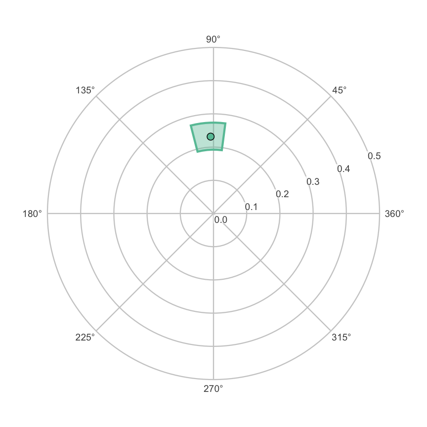

knitr::kable(
  ssm_table(latent, render = FALSE),
  caption = "Latent SSM profile of NARPD"
)

Latent SSM profile of NARPD
Profile	Elevation	X.Value	Y.Value	Amplitude	Displacement	Fit
NARPD	0.25 (0.21, 0.29)	-0.01 (-0.05, 0.03)	0.23 (0.19, 0.27)	0.23 (0.19, 0.27)	92.1 (82.5, 104.5)	0.975

By default ssm_sem() fits with a robust estimator (estimator = "MLR") and reports robust global fit indices, because circumplex scale scores are typically skewed and the naive chi-square over-rejects. The robust (sandwich) standard errors also feed the confidence intervals — for a reason that is the subject of the next section.

4. Where the confidence intervals come from

Amplitude and displacement are nonlinear functions of the model parameters: amplitude is a square root and displacement is an atan2. lavaan can attach a delta-method or bootstrap-percentile interval to any derived quantity, but for displacement those intervals are wrong in a way that is easy to miss. atan2 has a branch cut: a displacement near 0°/360° can produce an interval that has been unwrapped across the cut, or whose endpoints have sign-flipped, so a naive percentile interval straddling the boundary points the wrong way around the circle.

circumplex therefore never delegates amplitude or displacement intervals to lavaan — the reason the generated syntax refuses to define them. Instead it reuses the same machinery the observed bootstrap uses:

lavaan supplies only the point estimates and their covariance (or bootstrap replicates) of the model’s free parameters.
ssm_sem() draws from that covariance, maps each draw through the profile and the SSM transform, and obtains a replicate of every SSM parameter.
Those replicates go through the package’s existing interval assembly — percentile intervals for the linear parameters, and circular quantiles for displacement (centered on the circular mean, unwrapped, quantiled, and re-wrapped), with contrast intervals aligned to the estimate’s branch.

The result is that a latent displacement interval behaves correctly at the 0°/360° pole: it can straddle the boundary contiguously, and the point estimate always sits inside its own interval. This is the same architecture the Monte Carlo engine uses for observed profiles, with lavaan supplying the mean and covariance rather than resampling.

Two engines feed step 2, selected by ci_method:

"mvn" (default): draw from a multivariate normal centered at the estimates with the model’s (robust) covariance. Fast — one model fit plus vectorized draws.
"boot": refit the model on each bootstrap resample. Far more expensive, but it does not lean on asymptotic normality.

A coverage study across constructed populations (reported in the package’s design notes) found "mvn" well-calibrated at realistic sample sizes when the covariance is the robust sandwich — which is why robust SEs are the default. Under a misspecified fixed-angle model, plain (non-robust) SEs undercovered displacement; the sandwich restored nominal coverage. If you supply your own lavaan fit through ssm_sem_parameters() and intend to use "mvn", fit it with se = "robust.huber.white" so the propagated covariance stays valid.

5. What the parameters mean now

Disattenuation changes what two of the parameters mean, and the vignette would be misleading if it did not say so.

Fit. Under the scaled tier the latent profile is not forced to be a perfect cosine — the scales have different saturations — so a latent fit below 1 is informative: it measures how far the measure’s latent profile departs from a pure cosine wave, driven by differential saturation across scales (and, under the strict tier, by anisotropy in the factor covariance). What the latent fit removes, relative to the observed fit, is the contamination from reliability heterogeneity — not sampling error. Both the observed and the latent fit are population quantities that contain no sampling error at all; as estimates at a finite sample size, both remain noisy, so a latent fit of, say, .85 in a modest sample is not automatically substantive structure.

Displacement. Latent displacement is the first-harmonic direction of the saturation-modulated disattenuated profile. It is not simply “the measure’s angle in the latent space.” Heterogeneous saturations around the circle, or a general factor leaning into the plane, rotate it — with fit possibly staying high — exactly as they rotate the observed displacement. The latent layer’s contribution is the removal of the reliability modulation that additionally rotates the observed displacement; it does not remove the saturation modulation. That removal is why the observed and latent displacements in Section 3 differ, and it is the honest description of what d estimates here.

The interpretation aids you already know carry over unchanged. Amplitude is the gate for interpreting displacement: when the amplitude confidence interval’s lower bound sits too close to zero relative to its width, the profile has no well-defined direction and the displacement is not interpretable — the low-fit dashing on plots and the displacement caution in print() behave exactly as they do for observed profiles.

6. Two questions about group differences

When you have groups, there are two distinct estimands, and circumplex keeps them separate on purpose.

Two estimands for a group difference
Question	Estimand	Tool	Confounds
Do the groups’ measured profiles differ?	Observed contrast	ssm_analyze(contrast = TRUE)	Structural difference, differential reliability, and non-invariance are combined.
Do the groups’ constructs differ, granted the instrument measures the same thing in both?	Latent contrast	ssm_sem(contrast = TRUE)	Disattenuated and conditional on measurement invariance; not computed when invariance fails.

Neither is more correct in the abstract. The observed contrast answers a question about scores and is always available. The latent contrast answers a question about constructs, but only if the instrument behaves the same way in both groups — and when it does not, the honest answer is that the groups cannot be compared on the latent metric, not a number.

7. Invariance-gated latent contrasts

Before it computes a latent group contrast, ssm_sem() fits an invariance ladder — configural, then metric, then scalar — and tests each rung against the previous one with lavaan’s own nested-model test (the scaled difference test under the robust estimator). The latent measure-profile contrast requires metric invariance (equal saturations across groups); the latent mean contrast additionally requires scalar invariance. If the required rung is rejected, the contrast is not computed.

On real data this gate does its job. Comparing the NARPD profile across the Gender groups in jz2017 rejects metric invariance, so ssm_sem() returns each group’s separate profile and an explicit non-comparison verdict rather than a contrast:

set.seed(12345)
by_gender <- ssm_sem(
  jz2017,
  scales = scales,
  angles = octants(),
  measures = "NARPD",
  grouping = "Gender",
  contrast = TRUE,
  boots = 300
)
by_gender
#> 
#> # Latent (SEM-based) SSM
#> 
#> Measurement model:    scaled fixed-angle circumplex
#> Global fit (N = 1166, robust): chisq(34) = 287.272, p < 0.001 
#>          CFI = 0.938, RMSEA = 0.123, SRMR = 0.06
#> 
#> Invariance ladder (gate: metric, alpha = 0.05):
#>        rung   chisq df   cfi rmsea dchisq ddf       p
#>  configural 287.272 34 0.938 0.123     NA  NA        
#>      metric 337.356 48 0.927 0.112 54.781  14 < 0.001
#> Verdict: metric invariance rejected (Δχ²(14) = 54.78, p < 0.0001, alpha = 0.05): these groups cannot be compared on this instrument's latent metric.
#> The requested latent contrast was therefore not computed; the rows below are each group's separate (configural) latent profile. The observed-score contrast (ssm_analyze()) answers its own, different question and remains available.
#> 
#> # Profile [NARPD: Female]:
#> 
#>                Estimate   Lower CI   Upper CI
#> Elevation         0.198      0.141      0.252
#> X-Value          -0.023     -0.083      0.040
#> Y-Value           0.250      0.188      0.318
#> Amplitude         0.251      0.194      0.318
#> Displacement     95.206     81.443    110.519
#> Model Fit         0.966                      
#> 
#> 
#> # Profile [NARPD: Male]:
#> 
#>                Estimate   Lower CI   Upper CI
#> Elevation         0.313      0.243      0.376
#> X-Value           0.012     -0.046      0.076
#> Y-Value           0.199      0.146      0.250
#> Amplitude         0.199      0.147      0.257
#> Displacement     86.611     70.075    103.660
#> Model Fit         0.977

The invariance ladder is printed with the decision, and no contrast is rendered — ssm_plot_contrast() on this object would have nothing to draw. This is deliberate: there is no force = TRUE. If you have a principled partial-invariance model, fit it yourself and pass it to ssm_sem_parameters(), which computes the contrast from whatever multi-group fit you supply and leaves the comparability claim to you.

When invariance is not the obstacle — for example, contrasting two measures within one group, where no cross-group invariance is at stake — the contrast is computed and behaves like the observed contrast (second measure minus first, displacement differences via the circular branch machinery):

set.seed(12345)
contrast <- ssm_sem(
  jz2017,
  scales = scales,
  angles = octants(),
  measures = c("NARPD", "ASPD"),
  contrast = TRUE,
  boots = 500
)
contrast
#> 
#> # Latent (SEM-based) SSM
#> 
#> Measurement model:    scaled fixed-angle circumplex
#> Global fit (N = 1166, robust): chisq(22) = 317.867, p < 0.001 
#>          CFI = 0.935, RMSEA = 0.114, SRMR = 0.068
#> 
#> # Profile [NARPD]:
#> 
#>                Estimate   Lower CI   Upper CI
#> Elevation         0.248      0.210      0.295
#> X-Value          -0.009     -0.052      0.032
#> Y-Value           0.231      0.191      0.272
#> Amplitude         0.231      0.193      0.272
#> Displacement     92.119     82.715    103.513
#> Model Fit         0.974                      
#> 
#> 
#> # Profile [ASPD]:
#> 
#>                Estimate   Lower CI   Upper CI
#> Elevation         0.161      0.115      0.207
#> X-Value          -0.043     -0.092     -0.002
#> Y-Value           0.250      0.208      0.295
#> Amplitude         0.254      0.216      0.298
#> Displacement     99.732     90.351    111.188
#> Model Fit         0.978                      
#> 
#> 
#> # Contrast [ASPD - NARPD]:
#> 
#>                  Estimate   Lower CI   Upper CI
#> Δ Elevation        -0.087     -0.138     -0.044
#> Δ X-Value          -0.034     -0.084      0.019
#> Δ Y-Value           0.019     -0.028      0.066
#> Δ Amplitude         0.022     -0.025      0.066
#> Δ Displacement      7.613     -6.113     19.993
#> Δ Model Fit         0.003

ssm_plot_contrast(contrast)

The contrast block reports the difference in each SSM parameter with its confidence interval. As with the observed contrast, an elevation or amplitude difference whose interval excludes zero is a difference in that parameter; the displacement difference is reported on the estimate’s angular branch, so its interval endpoints can legitimately fall outside ±180° near the boundary while still containing the estimate.

8. When to trust it: limitations

The latent layer buys disattenuation at the price of a set of assumptions. The documentation states them; the vignette should too.

Model-conditional. Every latent quantity is conditional on the fixed-angle model being adequate. Read the global fit first. As a real-data benchmark, Wendt et al. (2019) reported RMSEA between .075 and .111 for the fixed-loading circumplex CFA across four large samples — a real but imperfect approximation (their model targets the octants’ own latent structure, not an external measure’s profile, so the number is a benchmark, not a like-for-like comparison). The example fits here are of the same order (RMSEA around .12) and should likewise be read as approximations, not exact structure.
Fixed angles are theoretical. Departures from the theoretical geometry load into misfit, not into the angles. Use cpm_fit() to examine geometry.
Latent-plane stationarity is assumed, not tested. The plane factors are fixed isotropic and orthogonal; anisotropic latent dispersion surfaces only as global misfit.
The scaled tier assumes the general factor is orthogonal to the plane. A true general-factor lean surfaces as misfit under the scaled tier; use the strict tier to model it.
Displacement and fit have the disattenuated meanings of Section 5, not the naive “angle in latent space” and “cosine-ness” readings.
Disattenuated correlations can be large. Removing attenuation moves correlations toward ±1; values at or beyond 1 signal misspecification and are refused rather than summarized.
Invariance gating is a modeling decision with a default test, not an oracle. The observed contrast remains available and answers its own question.

9. Relation to the literature

The nearest published models are the confirmatory factor analyses of the interpersonal circumplex itself. Wendt et al. (2019) fit a three-factor circumplex CFA with fixed unit-cosine plane loadings — the shape of this package’s strict tier — across four large samples, and found the fully dimensional model competitive with categorical and hybrid alternatives. Their estimand, though, is the latent structure of the octant scales and persons’ factor scores, not an external measure’s disattenuated profile; their model is context for the strict tier, not a validation target for the SSM estimand.

At the level of a single disattenuated correlation, Moss (2026) showed that treating reliability as a known constant collapses interval coverage (to roughly .35 in one scenario), whereas propagating reliability uncertainty restores nominal coverage. That is exactly the logic behind fitting the model and propagating its full covariance rather than plugging in reliability point estimates. One estimand caveat: Moss’s disattenuated correlation corrects both variables for unreliability, whereas the latent SSM here corrects only the scale side — the external measure remains an observed variable — so the two are relatives, not the same quantity.

Finally, the two model families in this package meet at a single point: at a general factor orthogonal to the plane, equal saturations, and equally spaced angles, the fixed-loading circumplex CFA coincides with the one-harmonic, equal-communality version of Browne’s (1992) circumplex model that cpm_fit() estimates. The SEM-based SSM sits on the fixed-angle side of that boundary; to cross to freely estimated angles, use cpm_fit().

References

Browne, M. W. (1992). Circumplex models for correlation matrices. Psychometrika, 57(4), 469–497.
Moss, J. (2026). Inference for disattenuated correlations. Applied Psychological Measurement. Advance online publication. https://doi.org/10.1177/01466216261440511
Wendt, L. P., Wright, A. G. C., Pilkonis, P. A., Nolte, T., Fonagy, P., Montague, P. R., Benecke, C., Krieger, T., & Zimmermann, J. (2019). The latent structure of interpersonal problems: Validity of dimensional, categorical, and hybrid models. Journal of Abnormal Psychology, 128(8), 823–839.
Zimmermann, J., & Wright, A. G. C. (2017). Beyond description in interpersonal construct validation: Methodological advances in the circumplex Structural Summary Approach. Assessment, 24(1), 3–23.