Evaluating Circumplex Structure • circumplex

library(circumplex)

1. Two questions to ask before interpreting an SSM analysis

The Structural Summary Method (SSM) condenses a circumplex profile into a few interpretable parameters: elevation, amplitude, displacement, and fit. That condensation rests on two assumptions that are testable but often left untested:

Does the instrument actually have circumplex structure? The SSM locates a profile on a circle whose positions are given by the scales’ theoretical angles. If the scales do not really form a circumplex — or sit at very different angles than the theory says — the summary is distorted before any profile is computed.
Are the confidence intervals trustworthy at your sample size and profile? Zimmermann and Wright (2017) showed that the accuracy of bootstrap SSM intervals depends on the sample size, the instrument’s correlation structure, and — for amplitude and displacement — on how differentiated the profile really is in the population. Intervals that are accurate for one construct in your table can be inaccurate for the construct printed directly below it.

This vignette shows how to answer both questions with cpm_fit() and fit_structure() (question 1) and ssm_ci_accuracy() (question 2), using the jz2017 dataset — the same sample of 1,166 undergraduates analyzed in Zimmermann and Wright (2017, Study 5), with octant scores on the IIP-SC and personality disorder (PD) scales from the PDQ-4+.

2. Does the instrument fit a circumplex?

Fitting the circular process model

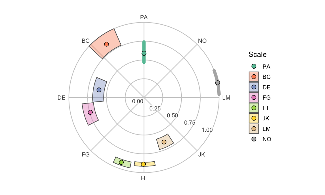
cpm_fit() estimates Browne’s (1992) circular process model (CPM), the confirmatory model behind the CIRCUM and CircE programs. Each scale gets an estimated angle on the circle and a communality index $\zeta$ (the correlation between the scale and the common circumplex “factor”; its square, $\zeta^2$ , is the scale’s communality — the share of its variance the circumplex explains). The model also yields the usual covariance-structure fit indices.

On the raw-data path the default confidence intervals are bootstrapped. We lower boots from its default of 2000 to keep this vignette quick to build; in practice, use the default.

data("jz2017")
set.seed(12345)
cpm <- cpm_fit(jz2017, scales = PANO(), angles = octants(), boots = 500)
#> Warning: CPM Hessian is ill-conditioned (condition number 1.83e+14): angles may
#> be clustered or parameters weakly determined.
#> Warning: 11 of 500 bootstrap resamples were excluded (0 with a degenerate or
#> non-positive-definite correlation matrix, 11 failing the convergence acceptance
#> criterion); the confidence intervals are based on the remaining 489 replicates
#> and are conditional on estimability.
summary(cpm)
#> 
#> Circular Process Model (Browne, 1992) 
#> Model:             quasi-circumplex 
#> Harmonics (m):     3 
#> Sample size (N):   1166 
#> Reference scale:   PA 
#> CI method:         bootstrap 
#> Confidence level:  0.95 
#> 
#> # Estimated angles and communality indices
#> 
#>  Scale Angle_theory   Angle Angle_lci Angle_uci  Zeta Zeta_lci Zeta_uci
#>     PA           90  90.000    90.000    90.000 0.767    0.684    0.860
#>     BC          135 125.074   113.548   137.069 0.931    0.872    1.000
#>     DE          180 170.353   156.943   185.174 0.780    0.733    0.826
#>     FG          225 195.425   185.811   206.523 0.861    0.822    0.910
#>     HI          270 250.721   244.660   258.758 0.956    0.935    0.977
#>     JK          315 269.491   261.813   279.412 0.942    0.929    0.957
#>     LM          360 294.230   286.626   303.019 0.806    0.761    0.850
#>     NO           45  11.305     2.426    20.913 1.000    1.000    1.000
#>  Communality
#>        0.589
#>        0.868
#>        0.608
#>        0.741
#>        0.914
#>        0.888
#>        0.650
#>        1.000
#> 
#> # Correlation-function weights
#> 
#>  k  Beta Beta_lci Beta_uci
#>  0 0.450    0.418    0.481
#>  1 0.440    0.411    0.466
#>  2 0.074    0.065    0.087
#>  3 0.036    0.015    0.057
#> 
#> # Fit indices
#> 
#>   χ²(10) = 81.169, p = <1e-04
#>   RMSEA = 0.078 [0.063, 0.094] (90% CI)
#>   SRMR  = 0.042
#>   CFI   = 0.984    TLI = 0.956
#>   AIC   = 117.169    BIC = 208.273
#> 
#> # Residuals
#> 
#>   Largest absolute residual: 0.134 (PA – HI)
#> 
#> # Diagnostics
#> 
#>   Note: a communality index reached its upper boundary (ζ > 0.995, a Heywood-type solution).
#>   Note: 11 of 500 bootstrap resamples were excluded (0 degenerate, 11 non-convergent); the intervals are based on 489 replicates and are conditional on estimability.

Two parts of this output matter most for evaluating structure:

The estimated angles. Compare them with the theoretical angles: the IIP-SC octants land near — but not exactly on — their theoretical positions, so the circumplex ordering is preserved while the spacing is not perfectly equal. This is the typical result for well-validated circumplex instruments: minor deviations from perfect structure are common and have little practical impact on SSM profiles (Gurtman & Pincus, 2000).
The communality indices. Scales with low $\zeta$ are poorly described by the circle; a profile peak at such a scale’s angle means less than the same peak at a well-explained scale’s angle.

The estimated configuration is easiest to read on the circle itself: each scale is drawn at its estimated angle, at a radius equal to its communality ( $\zeta^2$ ), with a joint confidence region where one is estimable.

plot(cpm)

Reading the fit indices

The summary() output reports the standard indices, and the standard benchmarks apply: RMSEA at or below about .08 suggests adequate approximate fit and above about .10 poor fit (Browne & Cudeck, 1993); SRMR at or below about .08 suggests acceptable average residuals (Hu & Bentler, 1999); CFI and TLI near .95 or above suggest good comparative fit (Hu & Bentler, 1999). Treat these as conventions from the broader covariance-structure literature, not circumplex-specific laws.

Two circumplex-specific cautions, both from this package’s own validation simulations:

Boundary solutions are common at realistic sample sizes. When octant scales share a strong general factor (as interpersonal problem scales do), fitted solutions frequently sit at or near a parameter boundary — a communality estimate at 1 (a “Heywood” case), or a harmonic weight at 0. cpm_fit() flags these in its diagnostics. They are usually a property of the estimator meeting real data at finite $n$ , not a data-entry error, but they matter for inference (next point).
Do not lean hard on the chi-square p value. In simulations at field-typical sample sizes with octant-like population structures, the test statistic did not follow its nominal chi-square reference distribution, even for correctly specified models. Read the chi-square descriptively (bigger is worse), and prefer RMSEA/SRMR/CFI for judging approximate fit.

For the same reasons, when the intervals are analytic (Wald) — the only option on the correlation-matrix input path — summary() prints a caution below $N = 2000$ , and up to very large $N$ when a boundary marker is present: in validation, analytic intervals mis-covered in exactly those regimes. Prefer the bootstrap (the raw-data default) when you have raw data.

Comparing model variants

Constrained variants make the structural question sharp: is the instrument consistent with equally spaced scales? With equal communalities? The correlation-matrix path is convenient for this comparison (point estimates and fit indices are deterministic, so no bootstrap is needed):

R <- cpm$matrices$R # the sample correlation matrix stored by cpm_fit()
fits <- lapply(
  c("quasi-circumplex", "equal-communality", "circulant"),
  function(mod) {
    cpm_fit(
      cormat = R, scales = PANO(), angles = octants(),
      n = nrow(jz2017), model = mod
    )
  }
)
#> Warning: CPM Hessian is ill-conditioned (condition number 1.83e+14): angles may
#> be clustered or parameters weakly determined.
data.frame(
  model = vapply(fits, function(f) f$details$model, character(1)),
  df = vapply(fits, function(f) f$fit$df, numeric(1)),
  rmsea = round(vapply(fits, function(f) f$fit$rmsea, numeric(1)), 3),
  srmr = round(vapply(fits, function(f) f$fit$srmr, numeric(1)), 3),
  cfi = round(vapply(fits, function(f) f$fit$cfi, numeric(1)), 3),
  tli = round(vapply(fits, function(f) f$fit$tli, numeric(1)), 3)
)
#>               model df rmsea  srmr   cfi   tli
#> 1  quasi-circumplex 10 0.078 0.042 0.984 0.956
#> 2 equal-communality 17 0.100 0.063 0.956 0.928
#> 3         circulant 24 0.185 0.130 0.790 0.755

The pattern reproduces what Zimmermann and Wright (2017, p. 14) reported for these data with CircE: the fully constrained model (equal spacing and equal communality — the "circulant" variant) fits poorly, while relaxing the equal-spacing constraint improves fit to the edge of the conventional benchmarks (marginal by RMSEA, acceptable by SRMR and CFI); they reported CFI = .824, TLI = .795, RMSEA = .169 for the former and CFI = .958, TLI = .931, RMSEA = .098 for the latter. Do not expect the default fit’s indices to match theirs to the digit: CIRCUM/CircE fit a covariance version of the model with free scaling constants, whereas cpm_fit() by default fits the correlation structure directly, and the two differ slightly at finite sample sizes; pass scaling = "free" to fit their covariance parameterization and reproduce published CIRCUM/CircE output exactly. For the model test the choice does not matter here: with correlation input the two families’ test statistics are calibration-indistinguishable (differing by well under 1% of the model degrees of freedom in paired simulation at sample sizes 250–50,000; the free statistic never exceeds the default’s on the same input beyond numerical tolerance, since the free family nests the default and is additionally started from its solution), and the default is recommended for routine inference because free scaling adds parameters whose analytic standard errors are often undefined at small-to-moderate samples. The conclusion — ordered octants with unequal spacing, adequate approximate fit once equal spacing is not forced — is the same.

A poor CPM fit does not make SSM output uncomputable; it makes the summary less meaningful, because the profile is being referred to scale positions the data contradict. If the ordering itself fails (scales out of sequence around the circle), SSM parameters should not be interpreted.

3. Can you trust your confidence intervals?

What Zimmermann & Wright (2017) found

Zimmermann and Wright’s simulation studies (their Studies 1–4) evaluated the accuracy of 95% percentile bootstrap intervals for SSM parameters — the same interval type ssm_analyze() reports — judging an interval accurate when its empirical coverage stayed within Bradley’s (1978) liberal band of 92.5% to 97.5%. Their headline results:

Parameter	Point estimate	95% bootstrap CI accurate when…
Elevation ( $e$ )	essentially unbiased	$n \ge 50$
X value / affiliation	essentially unbiased	$n \ge 50$
Y value / dominance	essentially unbiased	$n \ge 50$
Amplitude ( $a$ )	biased upward, strongly so when population amplitude is small	$n \ge 75$ (general-factor instrument) or $n \ge 150$ (no general factor), given population amplitude $\ge .10$
Displacement ( $\delta$ )	unbiased but imprecise at low amplitude	$n \ge 100$ (general factor) or $n > 200$ (no general factor), given population amplitude $\ge .10$
Fit ( $R^2$ )	biased downward	population $R^2 < .9$ only; unsuited near 1

(Transcribed from Zimmermann & Wright, 2017, Studies 1–2, pp. 6–11.)

Three implications are worth internalizing:

Amplitude overestimates differentiation. Across their conditions the relative bias averaged 15.5% and reached 135.8%; with $n = 50$ and no general factor, the expected sample amplitude was about .15 when the population amplitude was exactly zero (their pp. 6–7). An amplitude of .15 is commonly read as “marked”; at small $n$ it can be pure sampling artifact.
Displacement is only as stable as amplitude is large. The standard error of the displacement grows as amplitude shrinks (e.g., roughly 50 degrees at $n = 100$ for a weakly differentiated profile; their p. 8). A displacement estimate from a flat profile has no meaningful direction.
The thresholds above are grid minima, not guarantees. They come from specific instruments, specific sample sizes, and population amplitudes of .10 or larger. Their Study 3 quantified the frontier more finely: the minimum population affiliation/dominance component needed for accurate amplitude and displacement intervals is approximately $2.95 \cdot f_a \cdot n^{-0.587}$ , where $f_a$ is an instrument constant (their Eq. 3; ≈ .55 for the IIP-C, .63 for the IIP-SC, .85 for the IAS). At $n = 100$ with an IIP-C-like instrument that is a population component of about .11 — larger than many real construct profiles.

Simulating coverage for your own analysis

Published thresholds cover a coarse grid of conditions, and your analysis — your instrument, your $n$ , your group sizes, your profile, your number of bootstrap resamples — usually falls between or outside the grid points. ssm_ci_accuracy() answers the question directly at your configuration: it builds a population whose structure matches your fitted estimates (through the CPM by default), simulates many datasets of your exact sample size from it, replays your own CI procedure on each, and reports how often the intervals covered the known population values.

To see it catch a real problem, we analyze two PD scales at a modest sample size: paranoid PD (a well-differentiated interpersonal profile) and obsessive–compulsive PD, whose profile Zimmermann and Wright’s Table 4 showed to be nearly flat (amplitude .012 at full sample size). We use the first 250 participants — a sample size many construct-validation studies would consider respectable.

set.seed(23456)
res <- ssm_analyze(
  jz2017[1:250, ],
  scales = PANO(),
  angles = octants(),
  measures = c("PARPD", "OCPD"),
  boots = 500 # reduced from the default 2000 to keep the vignette quick;
  # the diagnostic below replays whatever procedure this object used
)
summary(res)
#> 
#> Statistical Basis:    Correlation Scores 
#> Bootstrap Resamples:  500 
#> Confidence Level:     0.95 
#> Listwise Deletion:    TRUE 
#> Scale Displacements:  90 135 180 225 270 315 360 45 
#> 
#> 
#> # Profile [PARPD]:
#> 
#>                Estimate   Lower CI   Upper CI
#> Elevation         0.258      0.169      0.338
#> X-Value          -0.095     -0.160     -0.028
#> Y-Value           0.055     -0.017      0.122
#> Amplitude         0.110      0.054      0.185
#> Displacement    149.667    111.480    190.360
#> Model Fit         0.725                      
#> 
#> 
#> # Profile [OCPD]:
#> 
#>                Estimate   Lower CI   Upper CI
#> Elevation         0.218      0.123      0.302
#> X-Value          -0.021     -0.084      0.037
#> Y-Value          -0.003     -0.068      0.063
#> Amplitude         0.021      0.009      0.096
#> Displacement    188.695     29.052    335.755
#> Model Fit         0.150                      
#>   Note: model fit is inadequate (R² < .70); interpret only the elevation parameter.
#>   Note: the amplitude CI lower bound is under 0.35 CI-widths above zero; the displacement is not interpretable.

Note the guardrail in the printed output: when a profile’s amplitude CI lower bound sits less than 0.35 CI-widths above zero, ssm_analyze() marks the displacement as uninterpretable rather than certifying its direction. That rule is scale-free (it compares the lower bound to the interval’s own width, so it means the same thing on any score metric) and does not depend on the display precision. The diagnostic below measures, among other things, how well that certification rule performs at your configuration.

We again use reduced settings (reps = 200, a short amplitude ladder, and the smaller boots above) to keep the vignette fast; the defaults (reps = 1000, four ladder rungs, on an object built with the default boots = 2000) give a Monte Carlo standard error under one percentage point for coverage near the nominal level and are recommended in practice. The parallel/ncpus arguments speed up real runs without changing results for a given seed.

set.seed(34567)
acc <- ssm_ci_accuracy(res, reps = 200, amplitude_factors = c(1, 0.5, 0))
#> Warning: CPM Hessian is ill-conditioned (condition number 9.17e+16): angles may
#> be clustered or parameters weakly determined.
summary(acc)
#> 
#> Statistical Basis:    Correlation Scores 
#> Assessed Engine:  bootstrap with 500 replicates 
#> Confidence Level:     0.95 
#> Simulation Reps:  200 per condition 
#> Amplitude Ladder:     1 0.5 0 2.077 
#> Population Structure:     Browne circular model (CPM) 
#> Group Sizes:      All = 250 
#> Certification Rule:   a_lci / (a_uci - a_lci) >= 0.35 (scale-free, print-independent) 
#> Elapsed:      14.1 s
#> 
#> Structure note: population simulated from a Browne circular model fit (m = 3,
#> RMSEA = 0.064, SRMR = 0.038).
#>   The structure fits adequately (RMSEA <= 0.08, Browne & Cudeck, 1993; SRMR
#>   <= 0.08, Hu & Bentler, 1999), so the simulated population is a reasonable
#>   stand-in for yours.
#>   Boundary markers: Heywood communality; small correlation-function weight;
#>   ill-conditioned Hessian.
#> Near-zero regime: the amplitude estimate of profile [OCPD] is below half its
#> own CI width, so your analysis already sits in the amplitude-near-zero
#> regime; an absolute rung at the certification margin (c = 2.08, population
#> amplitude = the observed CI half-width) was added to the ladder.
#> 
#> CI trustworthiness at the as-estimated condition (c = 1), classified
#> against Bradley's (1978) liberal band via 95% Wilson intervals:
#> 
#>   # Profile [PARPD] (n = 250; 95% bootstrap CIs, 500 replicates):
#>     Elevation      coverage 94.0% -- borderline
#>     Amplitude      coverage 94.0% -- borderline
#>     Displacement   coverage 89.6% when certified -- borderline
#>     Guardrail      under a truly zero amplitude, displacement would be
#>                    certified 1.0% of the time (user-expectation benchmark
#>                    2.5%)
#>   Verdict: BORDERLINE -- elevation, amplitude, and certified displacement
#>   coverage rates are borderline at this number of replications; a larger
#>   `reps` would sharpen the verdict.
#> 
#>   # Profile [OCPD] (n = 250; 95% bootstrap CIs, 500 replicates):
#>     Elevation      coverage 94.0% -- borderline
#>     Amplitude      coverage 85.0% -- INADEQUATE (under-coverage; misses are
#>                    almost all below the interval: the amplitude CI tends to
#>                    sit above the truth)
#>     Displacement   coverage 60.0% when certified -- INADEQUATE
#>                    (under-coverage)
#>     Guardrail      under a truly zero amplitude, displacement would be
#>                    certified 1.0% of the time (user-expectation benchmark
#>                    2.5%)
#>   Verdict: CAUTION -- amplitude CIs are less reliable than nominal at this
#>   sample size and displacement CIs mis-cover even when certified. Elevation
#>   coverage is borderline at this number of replications; a larger `reps`
#>   would sharpen the verdict. Consider a larger sample or treat near-zero
#>   amplitudes as inconclusive rather than absent.
#> 
#> Coverage by profile, parameter, and amplitude condition:
#>  Profile Parameter Condition Coverage MC_se Left_miss Right_miss Median_width
#>    PARPD         e     1.000    0.940 0.017     0.030      0.030        0.152
#>    PARPD         x     1.000    0.940 0.017     0.030      0.030        0.122
#>    PARPD         y     1.000    0.925 0.019     0.020      0.055        0.131
#>    PARPD         a     1.000    0.940 0.017     0.045      0.015        0.125
#>    PARPD         d     1.000    0.920 0.019     0.035      0.045       63.384
#>     OCPD         e     1.000    0.940 0.017     0.025      0.035        0.156
#>     OCPD         x     1.000    0.945 0.016     0.025      0.030        0.126
#>     OCPD         y     1.000    0.965 0.013     0.030      0.005        0.131
#>     OCPD         a     1.000    0.850 0.025     0.150      0.000        0.103
#>     OCPD         d     1.000    0.825 0.027     0.075      0.100      221.255
#>    PARPD         e     0.500    0.945 0.016     0.025      0.030        0.152
#>    PARPD         x     0.500    0.935 0.017     0.025      0.040        0.124
#>    PARPD         y     0.500    0.930 0.018     0.020      0.050        0.128
#>    PARPD         a     0.500    0.945 0.016     0.055      0.000        0.112
#>    PARPD         d     0.500    0.915 0.020     0.045      0.040      157.065
#>     OCPD         e     0.500    0.940 0.017     0.030      0.030        0.158
#>     OCPD         x     0.500    0.940 0.017     0.030      0.030        0.128
#>     OCPD         y     0.500    0.930 0.018     0.025      0.045        0.131
#>     OCPD         a     0.500    0.460 0.035     0.540      0.000        0.102
#>     OCPD         d     0.500    0.710 0.032     0.160      0.130      256.904
#>    PARPD         e     0.000    0.945 0.016     0.020      0.035        0.153
#>    PARPD         x     0.000    0.935 0.017     0.030      0.035        0.123
#>    PARPD         y     0.000    0.950 0.015     0.040      0.010        0.131
#>    PARPD         a     0.000    0.000 0.000     1.000      0.000        0.099
#>    PARPD         d     0.000       NA    NA        NA         NA           NA
#>     OCPD         e     0.000    0.915 0.020     0.040      0.045        0.157
#>     OCPD         x     0.000    0.960 0.014     0.030      0.010        0.125
#>     OCPD         y     0.000    0.945 0.016     0.020      0.035        0.132
#>     OCPD         a     0.000    0.000 0.000     1.000      0.000        0.101
#>     OCPD         d     0.000       NA    NA        NA         NA           NA
#>    PARPD         e     2.077    0.950 0.015     0.025      0.025        0.151
#>    PARPD         x     2.077    0.945 0.016     0.030      0.025        0.118
#>    PARPD         y     2.077    0.935 0.017     0.035      0.030        0.128
#>    PARPD         a     2.077    0.930 0.018     0.035      0.035        0.124
#>    PARPD         d     2.077    0.955 0.015     0.015      0.030       31.199
#>     OCPD         e     2.077    0.930 0.018     0.040      0.030        0.157
#>     OCPD         x     2.077    0.910 0.020     0.060      0.030        0.126
#>     OCPD         y     2.077    0.945 0.016     0.030      0.025        0.131
#>     OCPD         a     2.077    0.925 0.019     0.075      0.000        0.109
#>     OCPD         d     2.077    0.885 0.023     0.050      0.065      158.585
#>  Coverage_conditional N_conditional Structural N_reps
#>                    NA            NA      FALSE    200
#>                    NA            NA      FALSE    200
#>                    NA            NA      FALSE    200
#>                    NA            NA      FALSE    200
#>                 0.896           144      FALSE    200
#>                    NA            NA      FALSE    200
#>                    NA            NA      FALSE    200
#>                    NA            NA      FALSE    200
#>                    NA            NA      FALSE    200
#>                 0.600            10      FALSE    200
#>                    NA            NA      FALSE    200
#>                    NA            NA      FALSE    200
#>                    NA            NA      FALSE    200
#>                    NA            NA      FALSE    200
#>                 0.926            27      FALSE    200
#>                    NA            NA      FALSE    200
#>                    NA            NA      FALSE    200
#>                    NA            NA      FALSE    200
#>                    NA            NA      FALSE    200
#>                 0.000             3      FALSE    200
#>                    NA            NA      FALSE    200
#>                    NA            NA      FALSE    200
#>                    NA            NA      FALSE    200
#>                    NA            NA       TRUE    200
#>                    NA             0      FALSE      0
#>                    NA            NA      FALSE    200
#>                    NA            NA      FALSE    200
#>                    NA            NA      FALSE    200
#>                    NA            NA       TRUE    200
#>                    NA             0      FALSE      0
#>                    NA            NA      FALSE    200
#>                    NA            NA      FALSE    200
#>                    NA            NA      FALSE    200
#>                    NA            NA      FALSE    200
#>                 0.955           200      FALSE    200
#>                    NA            NA      FALSE    200
#>                    NA            NA      FALSE    200
#>                    NA            NA      FALSE    200
#>                    NA            NA      FALSE    200
#>                 0.882            17      FALSE    200
#>   Note: amplitude coverage on rows flagged Structural is structurally 0 (a
#>   percentile interval of strictly positive amplitude replicates cannot
#>   contain a zero truth) -- a theorem, not a measurement; the informative
#>   near-zero rungs are the small c > 0 ones.
#> 
#> Guardrail operating characteristics:
#>  Profile Condition Cert_rate Cert_lci Cert_uci Benchmark Caution Fit_pass_rate
#>    PARPD     1.000     0.720    0.654    0.778     0.025      NA         0.555
#>     OCPD     1.000     0.050    0.027    0.090     0.025      NA         0.075
#>    PARPD     0.500     0.135    0.094    0.189     0.025      NA         0.115
#>     OCPD     0.500     0.015    0.005    0.043     0.025      NA         0.045
#>    PARPD     0.000     0.010    0.003    0.036     0.025   FALSE         0.020
#>     OCPD     0.000     0.010    0.003    0.036     0.025   FALSE         0.070
#>    PARPD     2.077     1.000    0.981    1.000     0.025      NA         0.985
#>     OCPD     2.077     0.085    0.054    0.132     0.025      NA         0.115
#>  Branch_pathology_rate N_reps
#>                      0    200
#>                      0    200
#>                      0    200
#>                      0    200
#>                      0    200
#>                      0    200
#>                      0    200
#>                      0    200

How to read this output:

The coverage table reports, for each parameter, how often your CI procedure covered the truth in the simulated replications, at the amplitude the profile was estimated to have (Condition = 1) and at fractions of it. Compare coverage against the nominal level using the Wilson interval and the Bradley band, which is what the verdict does for you.
The amplitude ladder (Condition column) matters because your estimated amplitude is biased upward — the population that generated your data plausibly has less differentiation than your estimate. The rungs below 1 show what happens to coverage in that direction; the 0 rung shows the degenerate flat-profile case, where displacement has no true value at all and the amplitude interval cannot cover the boundary truth (its printed zero coverage is structural, flagged in the table). When a profile’s estimated amplitude is smaller than half its own CI width — as for obsessive–compulsive PD here — the diagnostic adds one more rung at a scaling factor above 1, the amplitude at which the population would sit exactly at the observed CI half-width.
The guardrail table reports how often profiles were certified (amplitude CI lower bound at least 0.35 CI-widths above zero) at each rung. At the 0 rung, any certification is a false certification: the summary prints a caution when the false-certification rate is materially above the rate a user would expect from the interval level. This is a measured property of the shipped display rule, not a hypothesis test.
The verdict classifies elevation, amplitude, and certification-conditional displacement coverage at your as-estimated amplitude, and the plain-language paragraph states the overall conclusion per profile.

For a visual summary across the ladder:

plot(acc)

The two profiles tell usefully different stories. Paranoid PD is certified: its amplitude CI lower bound clears the 0.35-CI-width margin, so ssm_analyze() reports its displacement, and nothing in its coverage table clearly leaves the Bradley band at the as-estimated amplitude or with the population amplitude halved. Obsessive–compulsive PD is not certified — its amplitude (about .02 here) is far too close to zero relative to its CI width — so the printed output already withholds its displacement as uninterpretable, before any coverage question is asked. On top of that, the diagnostic shows its amplitude and displacement CIs under-cover badly at this sample size (missing below the truth), so its verdict is a caution for a genuine reason: the intervals themselves are unreliable, not merely the point on the circle.

The guardrail line confirms the rule is doing its job. At this configuration ( $n = 250$ , eight octant correlations), a profile whose true amplitude is exactly zero would be certified only about the benchmark rate — roughly the one-sided error a user reading the guardrail would expect — so no caution fires from the guardrail itself. This is the scale-free rule’s payoff: unlike a fixed amplitude-unit cutoff, it holds false-certification near its intended rate even in the near-zero regime Zimmermann and Wright flagged, where a sample amplitude large enough to look non-zero is otherwise the expected outcome from a flat population.

One reading note: at reduced reps, classes tend to print as borderline — the Wilson interval around the estimated coverage is too wide to place it clearly inside or outside the Bradley band. That is the diagnostic being honest about its own Monte Carlo error; the default reps = 1000 sharpens such classifications into adequate or inadequate.

Two settings worth knowing: structure = "observed" rebuilds the population from the pooled observed correlations instead of the CPM — if the two structures yield different verdicts, that disagreement is itself informative (structure uncertainty is material for your data); and the embedded CPM fit is returned as acc$cpm for inspection with the tools from Section 2.

The diagnostic itself was validated against Zimmermann and Wright’s published results: configured to their transcribed simulation conditions, it reproduces their accuracy classifications — coverage inside the Bradley band at conditions they found accurate, and the same one-sided under-coverage at conditions they found inaccurate.

When to trust SSM parameters

Putting Sections 2 and 3 together into a checklist:

Structure first. Fit cpm_fit() to your instrument in your sample. If the octant ordering fails or communalities are very low, stop; SSM positions mean little.
Elevation is the robust parameter. Essentially unbiased, and its intervals were accurate from $n \ge 50$ in every published and package-run condition. (On the correlation path, elevation is also the parameter ipsatizing destroys — see Section 4.)
Treat amplitude as optimistic. It cannot go below zero, so it overshoots when true differentiation is weak. Before interpreting a “marked” amplitude at modest $n$ , run ssm_ci_accuracy() and look at the sub-1 ladder rungs.
Only interpret displacement when amplitude is credible. The package already withholds the displacement interval when the amplitude CI lower bound sits less than 0.35 CI-widths above zero; the diagnostic tells you how reliable that certification is at your configuration.
Do not build claims on the fit parameter’s interval. Zimmermann and Wright found bootstrap $R^2$ intervals accurate only when population fit was mediocre — near-perfect prototypicality cannot be bracketed from below. Report $R^2$ descriptively.
Remember what the diagnostic conditions on. It asks “would my CI procedure work in a population like my estimates”, under multivariate normality, with complete data. It is a strong check, not a certificate.

4. Does the instrument have circumplex structure at all?

Section 2’s confirmatory model (cpm_fit()) fits one theory-driven circular model and asks how well it fits. A complementary, more exploratory question is whether the scales’ correlations show circumplex structure at all, without committing to the theoretical angles: are the scales spread evenly around a circle, with comparable communalities, rather than clustering into a small number of independent clusters (simple structure)? Acton and Revelle (2004) evaluated ten such criteria by simulation; fit_structure() implements four of them — Fisher, Gap, VT2, and Rotation — leaving out a variance-test variant A&R found ineffective (VT1) and a criterion so highly correlated with Rotation as to be redundant (MT, r = .99 with RT in their Table 1). A fifth test, RANDALL, is not one of A&R’s ten at all: it is an independent order-correspondence test (Hubert & Arabie, 1987; Tracey, 1997) that A&R excluded from their own simulation because, unlike their criteria, its null distribution is known analytically rather than needing simulated cutoffs (their footnote 3).

The five tests

fit_structure() extracts the first two unrotated principal-axis factors of the scales’ correlation matrix (Acton & Revelle, 2004, p. 13) and computes four criteria from that two-factor solution, plus a fifth test that works directly on the correlations:

Fisher Test (equal axes). Are the scales’ communalities on the two-factor solution comparable, rather than one axis dominating? The statistic is the coefficient of variation of the scales’ vector lengths $\sqrt{h^2}$ .
Gap Test (equal spacing). Are the scales evenly distributed in angle around the circle, rather than bunched together? The statistic is the variance of the angular gaps between angularly adjacent scales, including the gap that wraps from the last scale back around to the first.
Variance Test (VT2) and Rotation Test (interstitiality). Both ask whether the scales sit between a small number of dominant axes rather than on them — the signature of a genuine circumplex, as opposed to simple structure. Each takes a criterion computed at many rotations of the two-factor solution and summarizes it as a coefficient of variation across rotations; a true circumplex is indifferent to rotation, so both criteria stay low.
RANDALL (Hubert & Arabie, 1987; Tracey, 1997). Does the hypothesized circular order you supplied (the order of scales) match the observed correlations, in the sense that closer-together scales correlate more strongly? Unlike the other four, this is a genuine randomization test: its null distribution (scales randomly relabeled onto the hypothesized positions) is enumerated exactly for up to nine scales, or estimated by Monte Carlo relabeling for more, so it returns an exact or Monte Carlo p value rather than a simulated cutoff.

The four factor-analytic criteria (Fisher, Gap, VT2, Rotation) have the most power to detect simple structure when there is no large general factor across the scales. Deviation scoring — centering each respondent on their own mean across the selected scales, exactly what ipsatize() does — approximates removing that general factor (Acton & Revelle, 2004, p. 9), so it is fit_structure()’s default; pass scoring = "raw" to analyze the scores as given. Each of the two scorings carries its own set of cutoffs (next section), matched automatically.

res <- fit_structure(jz2017, scales = PANO())
res
#> 
#> Circumplex Structure Tests (Acton & Revelle, 2004)
#> Scales (nv):  8
#> Scoring:      deviation (row-mean centered)
#> 
#> # Exploratory criteria
#> 
#>  Test     Statistic Interpretation                                           
#>  Fisher   0.102     equal axes: at least 3x as likely as the alternative     
#>  Gap      0.152     equal spacing: at least 3x as likely as the alternative  
#>  Variance 0.180     interstitiality: almost certain                          
#>  Rotation 0.325     interstitiality: at least 3x as likely as the alternative
#> 
#> # Order hypothesis (RANDALL)
#> 
#>   Correspondence index = 0.868, p = 0.000397 (exact, 5040 relabelings)
#> 
#>   Interpretations are heuristic likelihood classifications from simulation, not
#>   significance tests (Acton & Revelle, 2004). RANDALL's p-value is exact.

summary(res)
#> 
#> Circumplex Structure Tests (Acton & Revelle, 2004)
#> Scales (nv):  8
#> Scoring:      deviation (row-mean centered)
#> Ridge:        0
#> 
#> # Exploratory criteria
#> 
#>  Test     Statistic Almost Thrice Twice Verdict       
#>  Fisher   0.102     0.07   0.12   0.15  3x+ likely    
#>  Gap      0.152     0.15   0.40   0.46  3x+ likely    
#>  Variance 0.180     0.19   0.59   0.64  almost certain
#>  Rotation 0.325     0.32   0.64   0.67  3x+ likely    
#> 
#> # Estimated scale geometry
#> 
#>  Scale Angle   Communality
#>  PA    339.635 0.642      
#>  BC    359.858 0.571      
#>  DE     48.584 0.500      
#>  FG     81.337 0.522      
#>  HI    161.662 0.690      
#>  JK    183.339 0.713      
#>  LM    215.503 0.388      
#>  NO    287.119 0.474      
#> 
#> # Order hypothesis (RANDALL)
#> 
#>   Correspondence index = 0.868, p = 0.000397 (exact, 5040 relabelings)
#> 
#>   Interpretations are heuristic likelihood classifications from simulation, not
#>   significance tests (Acton & Revelle, 2004). RANDALL's p-value is exact.

summary() adds the numeric cutoffs behind each classification and the estimated angle and communality of every scale on the two-factor solution — the same geometry the plot below draws. A clean circumplex shows scales at roughly the theoretical octant spacing with broadly similar communalities; Fisher measures departures in communality, Gap/VT2/Rotation measure departures in even angular spread.

plot(res)

For the IIP-SC octants the picture agrees with Section 2’s CPM fit: the scales keep their theoretical circular ordering with comparable communalities and roughly even spacing, and the Fisher, Gap, and interstitiality criteria all classify the configuration as consistent with (or close to) a circumplex under deviation scoring. One caveat when reading the angles: the two-factor solution is unrotated, so its absolute orientation is arbitrary — it is the scales’ ordering and relative spacing that agree with theory, not their absolute angles (which is why summary() places PA well away from its nominal 90°). RANDALL’s p value confirms the hypothesized circular order directly, independent of the factor-analytic criteria.

Where the cutoffs come from

The four factor-analytic criteria are only as good as the thresholds used to classify them, and this is where the published article cannot be used as-is. Acton and Revelle calibrated their cutoffs by simulation at 64 and 128 variables and reported (their p. 18) that the Gap Test’s cutoffs shift sharply with the number of scales — far too sharply to reuse at the eight scales a typical circumplex instrument has. This package’s development process re-derived every cutoff at $n_v = 8$ under Acton and Revelle’s own generating model (their Eqs. 11.1–11.3), in a script committed at data-raw/structure-test-cutoffs.R: it first reproduced their published 64/128-variable design as a sanity gate on the simulation machinery, then reran the same design at $n_v = 8$ to derive the constants fit_structure() actually uses. The nv effect the re-derivation found is large — the raw- scored Gap Test’s “almost certain” cutoff moves from .01 at $n_v = 64/128$ to .35 at $n_v = 8$ — which is exactly why fit_structure() refuses to interpret any scale count it has not calibrated: at any $n_v \ne 8$ the statistics are still reported, but the classification column prints a dash rather than guessing.

RANDALL needs no such calibration; its p value comes from enumerating (or Monte Carlo sampling) the randomization null directly on your data, so it is available at any scale count of four or more.

Reading the classifications

The classification categories describe where a statistic falls among the simulated distributions for competing structures (circumplex vs. simple structure): “almost certain” (below the 1st percentile of the competing distribution), “at least 3x/2x as likely as the alternative” (the criterion’s structure is at least three/two times as likely as its competitor at that statistic value), and “not clearly supported”. Those ratios are likelihood ratios, not posterior probabilities or p values. They are heuristic classifications read off simulated distributions, not significance tests, and fit_structure()’s print()/summary() output repeats that caveat every time an interpretation is shown. Treat a “weak” or unsupported classification as a caution to inspect the loading configuration (the plot above) and Section 2’s CPM fit together, not as a rejection of any specific hypothesis.

How this complements the CPM fit

cpm_fit() (Section 2) and fit_structure() ask related but different questions. cpm_fit() commits to the theoretical angles and communality model and tests goodness of fit against that specific structure; a good overall RMSEA/CFI can still hide unequal spacing or a dominant general factor, both of which fit_structure() is built to detect. Conversely, fit_structure()’s exploratory criteria say nothing about how well the scales match your theoretical angles — only RANDALL, via the order you supply, references a hypothesis at all, and even that is an order hypothesis, not the specific angles cpm_fit() estimates. Running both is more informative than either alone: agreement between a good CPM fit and circumplex-supporting fit_structure() classifications is stronger evidence than either result on its own, and disagreement (for example, adequate CPM fit alongside a Fisher Test flagging unequal axes) points to exactly which aspect of circumplex structure to examine further.

5. Ipsatization and what it costs

Ipsatizing — subtracting each respondent’s own mean across the octant scales from each of their scale scores (ipsatize()) — is a common preprocessing step in circumplex work, used to remove individual differences in overall endorsement before examining profile shape.

For SSM analyses its main cost is simple to state: ipsatizing discards elevation. After row-centering, every respondent’s octant scores sum to zero, so a group’s mean profile has zero mean by construction, and the covariances between the ipsatized scales and any external measure sum to exactly zero — forcing the mean correlation toward zero regardless of how strongly the construct relates to the instrument’s general factor (Zimmermann & Wright, 2017, p. 4).

set.seed(45678)
res_raw <- ssm_analyze(
  jz2017,
  scales = PANO(),
  angles = octants(),
  measures = "PARPD",
  boots = 100
)
jz_ips <- ipsatize(jz2017, items = PANO())
set.seed(45678)
res_ips <- ssm_analyze(
  jz_ips,
  scales = paste0(PANO(), "_i"),
  angles = octants(),
  measures = "PARPD",
  boots = 100
)
comparison <- rbind(
  res_raw$results[, c("e_est", "a_est", "d_est")],
  res_ips$results[, c("e_est", "a_est", "d_est")]
)
rownames(comparison) <- c("raw", "ipsatized")
round(comparison, 3)
#>           e_est a_est   d_est
#> raw       0.250 0.150 128.945
#> ipsatized 0.007 0.113 132.949

The raw-score elevation — which matches the value Zimmermann and Wright report for this scale in their Table 4 — collapses to near zero after ipsatizing. The displacement stays close to its raw-score value, and the amplitude stays broadly similar — though not identical, because ipsatizing also changes the scales’ variances and intercorrelations, so shape parameters shift somewhat too. Guidance:

If elevation carries meaning in your application (for interpersonal problems it indexes association with generalized interpersonal distress), analyze raw scores and let the SSM separate elevation from shape — that separation is exactly what the model is for.
If you receive data that were already ipsatized, do not interpret the elevation row, and say so in the write-up; amplitude and displacement remain interpretable.
Do not describe an ipsatized profile’s near-zero elevation as evidence that a construct is “not generally interpersonal” — the preprocessing made that value uninformative.

6. Wrap-up

Evaluating circumplex structure has two layers: whether the instrument behaves like a circumplex in your sample (cpm_fit()), and whether the inferential machinery of the SSM can be trusted at your sample size and profile (ssm_ci_accuracy()). Both are one function call, and both change what you should claim more often than users expect — amplitude and displacement intervals, in particular, earn their trust only when the profile is genuinely differentiated relative to the precision your sample size affords.

References

Acton, G. S., & Revelle, W. (2004). Evaluation of ten psychometric criteria for circumplex structure. Methods of Psychological Research Online, 9(1), 1–27.
Bradley, J. V. (1978). Robustness? British Journal of Mathematical and Statistical Psychology, 31(2), 144–152.
Browne, M. W. (1992). Circumplex models for correlation matrices. Psychometrika, 57(4), 469–497.
Browne, M. W., & Cudeck, R. (1993). Alternative ways of assessing model fit. In K. A. Bollen & J. S. Long (Eds.), Testing structural equation models (pp. 136–162). Newbury Park, CA: Sage.
Grassi, M., Luccio, R., & Di Blas, L. (2010). CircE: An R implementation of Browne’s circular stochastic process model. Behavior Research Methods, 42(1), 55–73.
Gurtman, M. B., & Pincus, A. L. (2000). Interpersonal Adjective Scales: Confirmation of circumplex structure from multiple perspectives. Personality and Social Psychology Bulletin, 26(3), 374–384.
Hu, L., & Bentler, P. M. (1999). Cutoff criteria for fit indexes in covariance structure analysis: Conventional criteria versus new alternatives. Structural Equation Modeling, 6(1), 1–55.
Hubert, L., & Arabie, P. (1987). Evaluating order hypotheses within proximity matrices. Psychological Bulletin, 102(1), 172–178.
Tracey, T. J. G. (1997). RANDALL: A Microsoft FORTRAN program for a randomization test of hypothesized order relations. Educational and Psychological Measurement, 57(1), 164–168.
Zimmermann, J., & Wright, A. G. C. (2017). Beyond description in interpersonal construct validation: Methodological advances in the circumplex Structural Summary Approach. Assessment, 24(1), 3–23.