Confidence Interval Accuracy • circumplex

library(circumplex)

Level: Intermediate. Read “Evaluating Circumplex Structure” first.

1. Overview

This vignette asks whether the confidence intervals of an SSM analysis can be trusted at your sample size and profile. Section 2, “What Zimmermann & Wright (2017) found”, transcribes the published accuracy thresholds. Section 3, “Simulating coverage for your own analysis”, runs ssm_ci_accuracy() at your configuration and reads its report. Section 4, “When to trust SSM parameters”, puts the structure and accuracy checks into one checklist. The examples use the jz2017 dataset that “Evaluating Circumplex Structure” describes. The Wrap-up lists what the page covered and names the next page, and the References list the sources cited.

2. What Zimmermann & Wright (2017) found

Zimmermann and Wright’s simulation studies (their Studies 1–4) evaluated the accuracy of 95% percentile bootstrap intervals for SSM parameters. This is the same interval type that ssm_analyze() reports. They judged an interval accurate when its empirical coverage stayed within Bradley’s (1978) liberal band of 92.5% to 97.5%. Their headline results:

Parameter	Point estimate	95% bootstrap CI accurate when…
Elevation ( $e$ )	essentially unbiased	$n \ge 50$
X value / affiliation	essentially unbiased	$n \ge 50$
Y value / dominance	essentially unbiased	$n \ge 50$
Amplitude ( $a$ )	biased upward, strongly so when population amplitude is small	$n \ge 75$ (general-factor instrument) or $n \ge 150$ (no general factor), given population amplitude $\ge .10$
Displacement ( $\delta$ )	unbiased but imprecise at low amplitude	$n \ge 100$ (general factor) or $n > 200$ (no general factor), given population amplitude $\ge .10$
Fit ( $R^2$ )	biased downward	population $R^2 < .9$ only (unsuited near 1)

(Transcribed from Zimmermann & Wright, 2017, Studies 1–2, pp. 6–11.)

Three implications are worth internalizing:

Amplitude overestimates differentiation. Across their conditions, the relative bias averaged 15.5% and reached 135.8%. With $n = 50$ and no general factor, the expected sample amplitude was about .15 when the population amplitude was exactly zero (their pp. 6–7). An amplitude of .15 is commonly read as “marked”. At small $n$ , it can be pure sampling artifact.
Displacement is only as stable as amplitude is large. The standard error of the displacement grows as amplitude shrinks. For example, it is roughly 50 degrees at $n = 100$ for a weakly differentiated profile (their p. 8). A displacement estimate from a flat profile has no meaningful direction.
The thresholds above are grid minima, not guarantees. They come from specific instruments, specific sample sizes, and population amplitudes of .10 or larger. Their Study 3 quantified the frontier more finely. The minimum population affiliation/dominance component needed for accurate amplitude and displacement intervals is approximately $2.95 \cdot f_a \cdot n^{-0.587}$ . Here $f_a$ is an instrument constant (their Eq. 3). $f_a$ is about .55 for the IIP-C, .63 for the IIP-SC and .85 for the IAS. At $n = 100$ with an IIP-C-like instrument, that is a population component of about .11. That is larger than many real construct profiles.

3. Simulating coverage for your own analysis

Published thresholds cover a coarse grid of conditions. Your analysis (your instrument, your $n$ , your group sizes, your profile, your number of bootstrap resamples) usually falls between or outside the grid points. ssm_ci_accuracy() answers the question directly at your configuration. It builds a population whose structure matches your fitted estimates (through the CPM by default). It simulates many datasets of your exact sample size from that population, and it replays your own CI procedure on each. Then it reports how often the intervals covered the known population values.

To see it catch a real problem, we analyze two PD scales at a modest sample size. Paranoid PD has a well-differentiated interpersonal profile. Obsessive–compulsive PD has a profile that Zimmermann and Wright’s Table 4 showed to be nearly flat (amplitude .012 at full sample size). We use the first 250 participants. Many construct-validation studies would consider that sample size respectable.

set.seed(23456)
res <- ssm_analyze(
  jz2017[1:250, ],
  scales = PANO(),
  angles = octants(),
  measures = c("PARPD", "OCPD"),
  boots = 500 # reduced from the default 2000 to keep the vignette quick;
  # the diagnostic below replays whatever procedure this object used
)
summary(res)
#> 
#> Statistical Basis:    Correlation Scores 
#> Bootstrap Resamples:  500 
#> Confidence Level:     0.95 
#> Listwise Deletion:    TRUE 
#> Scale Displacements:  90 135 180 225 270 315 360 45 
#> 
#> 
#> # Profile [PARPD]:
#> 
#>                Estimate   Lower CI   Upper CI
#> Elevation         0.258      0.169      0.338
#> X-Value          -0.095     -0.160     -0.028
#> Y-Value           0.055     -0.017      0.122
#> Amplitude         0.110      0.054      0.185
#> Displacement    149.667    111.480    190.360
#> Model Fit         0.725                      
#> 
#> 
#> # Profile [OCPD]:
#> 
#>                Estimate   Lower CI   Upper CI
#> Elevation         0.218      0.123      0.302
#> X-Value          -0.021     -0.084      0.037
#> Y-Value          -0.003     -0.068      0.063
#> Amplitude         0.021      0.009      0.096
#> Displacement    188.695     29.052    335.755
#> Model Fit         0.150                      
#>   Note: model fit is inadequate (R² < .70); interpret only the elevation
#>   parameter.
#>   Note: the amplitude CI lower bound is under 0.35 CI-widths above zero; the
#>   displacement is not interpretable.

Note the guardrail in the printed output. When a profile’s amplitude CI lower bound sits less than 0.35 CI-widths above zero, ssm_analyze() marks the displacement as uninterpretable, rather than certifying its direction. That rule is scale-free. It compares the lower bound to the interval’s own width, so it means the same thing on any score metric. It also does not depend on the display precision. The diagnostic below measures, among other things, how well that certification rule performs at your configuration.

We again use reduced settings to keep the vignette fast: reps = 200, a short amplitude ladder, and the smaller boots above. The ladder is a set of scaling factors applied to the estimated amplitude (1 = as estimated), explained below. The defaults are reps = 1000 and four ladder rungs, on an object built with the default boots = 2000. They give a Monte Carlo standard error under one percentage point for coverage near the nominal level, and they are recommended in practice. The parallel/ncpus arguments speed up real runs without changing results for a given seed. The CPM fit inside the diagnostic prints the same ill-conditioned Hessian warning that “CPM Fits at a Boundary” explains.

print() shows the short report: one block of verdicts per profile.

set.seed(34567)
acc <- ssm_ci_accuracy(res, reps = 200, amplitude_factors = c(1, 0.5, 0))
#> Warning: CPM Hessian is ill-conditioned (condition number 9.24e+16): angles
#> may be clustered or parameters weakly determined.
print(acc)
#> 
#> SSM CI accuracy, simulated at your n and settings (200 replications per
#> condition; bootstrap intervals with 500 replicates at level 0.95)
#> 
#>   # Profile [PARPD] (n = 250; 95% bootstrap CIs, 500 replicates):
#>     Elevation      coverage 93.0%: borderline
#>     Amplitude      coverage 94.5%: borderline
#>     Displacement   coverage 89.1% when certified: borderline
#>     Guardrail      under a truly zero amplitude, displacement would be
#>                    certified 1.0% of the time (user-expectation benchmark
#>                    2.5%)
#>   Verdict: BORDERLINE. Elevation, amplitude, and certified displacement
#>   coverage rates are borderline at this number of replications; a larger
#>   `reps` would sharpen the verdict.
#> 
#>   # Profile [OCPD] (n = 250; 95% bootstrap CIs, 500 replicates):
#>     Elevation      coverage 95.0%: borderline
#>     Amplitude      coverage 83.0%: INADEQUATE (under-coverage; misses are
#>                    almost all below the interval: the amplitude CI tends to
#>                    sit above the truth)
#>     Displacement   coverage 50.0% when certified: INADEQUATE (under-coverage)
#>     Guardrail      under a truly zero amplitude, displacement would be
#>                    certified 1.0% of the time (user-expectation benchmark
#>                    2.5%)
#>   Verdict: CAUTION. Amplitude CIs are less reliable than nominal at this
#>   sample size and displacement CIs mis-cover even when certified. Elevation
#>   coverage is borderline at this number of replications; a larger `reps`
#>   would sharpen the verdict. Consider a larger sample or treat near-zero
#>   amplitudes as inconclusive rather than absent.

How to read this output. Each profile’s lines classify its coverage at the amplitude it was estimated to have. Coverage is how often your CI procedure covered the truth in the simulated replications. The diagnostic compares it with the nominal level, using the Wilson interval (an interval around the estimated coverage) and the Bradley band.

Elevation, Amplitude and Displacement give the coverage of each parameter and its class. Displacement coverage counts only the replications in which the profile was certified. A certified profile has its amplitude CI lower bound at least 0.35 CI-widths above zero.
Guardrail gives the rate at which a profile whose true amplitude is zero would still be certified. Any such certification is a false certification. The line prints a caution when that rate is materially above the rate that a user would expect from the interval level. This is a measured property of the shipped display rule, not a hypothesis test.
Verdict states the overall conclusion for the profile.

The two profiles tell usefully different stories. Paranoid PD is certified. Its amplitude CI lower bound clears the 0.35-CI-width margin, so the printed output adds no displacement note. None of its coverage rates clearly leaves the Bradley band at the as-estimated amplitude. Obsessive–compulsive PD is not certified. Its amplitude (about .02 here) is far too close to zero relative to its CI width. So the printed output still shows its displacement and interval, but with a note that the displacement is not interpretable. The ssm_analyze() result flags this on its own, before any coverage question is asked. On top of that, the diagnostic shows that its amplitude and displacement CIs under-cover badly at this sample size. Almost all amplitude misses fall below the interval, so the amplitude CI tends to sit above the truth. So its verdict is a caution for a genuine reason. The intervals themselves are unreliable, not merely the point on the circle.

The guardrail line confirms that the rule is doing its job. At this configuration ( $n = 250$ , eight octant correlations), take a profile whose true amplitude is exactly zero. Its estimated certification rate does not clearly exceed the benchmark rate. That rate is roughly the one-sided error that a user reading the guardrail would expect. So no caution fires from the guardrail itself. This is the payoff of the scale-free rule. Unlike a fixed amplitude-unit cutoff, it keeps false-certification from clearly exceeding the benchmark, even in the near-zero regime that Zimmermann and Wright flagged. In that regime, a sample amplitude large enough to look non-zero is otherwise the expected outcome from a flat population.

One reading note: at reduced reps, classes tend to print as borderline. This is because the Wilson interval around the estimated coverage is too wide to place it clearly inside or outside the Bradley band. That is the diagnostic being honest about its own Monte Carlo error. The default reps = 1000 sharpens such classifications into adequate or INADEQUATE.

The full report

summary() adds the settings, a note on the simulated population, and a table of coverage at every rung of the amplitude ladder:

summary(acc)
#> 
#> Correlation scores; bootstrap, 500 replicates, level 0.95; 200 reps per
#> condition.
#> Population: Browne circular model (CPM); groups All = 250; elapsed 11.7s.
#> Ladder c = 1, 0.5, 0, 2.077; certified if a_lci / (a_uci - a_lci) >= 0.35.
#> 
#> Structure note: population simulated from a Browne circular model fit (m = 3,
#> RMSEA = 0.064, SRMR = 0.038).
#>   The structure fits adequately (RMSEA <= 0.08, Browne & Cudeck, 1993; SRMR
#>   <= 0.08, Hu & Bentler, 1999), so the simulated population is a reasonable
#>   stand-in for yours.
#>   Boundary markers: Heywood communality; small correlation-function weight;
#>   ill-conditioned Hessian.
#> Near-zero regime: the amplitude estimate of profile [OCPD] is below half its
#> own CI width, so your analysis already sits in the amplitude-near-zero
#> regime; an absolute rung at the certification margin (c = 2.08, population
#> amplitude = the observed CI half-width) was added to the ladder.
#> 
#> Verdicts (c = 1, as estimated), Bradley (1978) liberal band, 95% Wilson CIs:
#> 
#>   # Profile [PARPD] (n = 250; 95% bootstrap CIs, 500 replicates):
#>     Elevation      coverage 93.0%: borderline
#>     Amplitude      coverage 94.5%: borderline
#>     Displacement   coverage 89.1% when certified: borderline
#>     Guardrail      under a truly zero amplitude, displacement would be
#>                    certified 1.0% of the time (user-expectation benchmark
#>                    2.5%)
#>   Verdict: BORDERLINE. Elevation, amplitude, and certified displacement
#>   coverage rates are borderline at this number of replications; a larger
#>   `reps` would sharpen the verdict.
#> 
#>   # Profile [OCPD] (n = 250; 95% bootstrap CIs, 500 replicates):
#>     Elevation      coverage 95.0%: borderline
#>     Amplitude      coverage 83.0%: INADEQUATE (under-coverage; misses are
#>                    almost all below the interval: the amplitude CI tends to
#>                    sit above the truth)
#>     Displacement   coverage 50.0% when certified: INADEQUATE (under-coverage)
#>     Guardrail      under a truly zero amplitude, displacement would be
#>                    certified 1.0% of the time (user-expectation benchmark
#>                    2.5%)
#>   Verdict: CAUTION. Amplitude CIs are less reliable than nominal at this
#>   sample size and displacement CIs mis-cover even when certified. Elevation
#>   coverage is borderline at this number of replications; a larger `reps`
#>   would sharpen the verdict. Consider a larger sample or treat near-zero
#>   amplitudes as inconclusive rather than absent.
#> 
#> Coverage by condition (d_cert: d when certified; cert: certification rate):
#>  Profile Condition     e     x     y     a     d d_cert  cert Structural
#>    PARPD     1.000 0.930 0.940 0.930 0.945 0.920  0.891 0.735      FALSE
#>    PARPD     0.500 0.945 0.935 0.935 0.935 0.905  0.893 0.140      FALSE
#>    PARPD     0.000 0.940 0.935 0.950 0.000    NA     NA 0.010       TRUE
#>    PARPD     2.077 0.945 0.950 0.935 0.930 0.955  0.955 1.000      FALSE
#>     OCPD     1.000 0.950 0.945 0.965 0.830 0.830  0.500 0.040      FALSE
#>     OCPD     0.500 0.940 0.940 0.935 0.485 0.710  0.333 0.015      FALSE
#>     OCPD     0.000 0.920 0.955 0.945 0.000    NA     NA 0.010       TRUE
#>     OCPD     2.077 0.930 0.915 0.945 0.930 0.885  0.833 0.090      FALSE
#>   Note: amplitude coverage on rows flagged Structural is structurally 0 (a
#>   percentile interval of strictly positive amplitude replicates cannot
#>   contain a zero truth). This is a theorem, not a measurement; the
#>   informative near-zero rungs are the small c > 0 ones.

How to read the additions:

The structure note describes the population the replications were drawn from, with its fit indices and any boundary markers from the CPM fit.
The coverage table reports coverage for each parameter at each rung of the ladder (Condition = 1 is the amplitude as estimated). The d_cert column is displacement coverage when certified.
The amplitude ladder (Condition column) matters because your estimated amplitude is biased upward. The population that generated your data plausibly has less differentiation than your estimate. The rungs below 1 show what happens to coverage in that direction. For paranoid PD, no coverage rate clearly leaves the Bradley band with the population amplitude halved either. The 0 rung shows the degenerate flat-profile case. There, displacement has no true value at all, and the amplitude interval cannot cover the boundary truth. (Its printed zero coverage is structural, and the table flags it.) When a profile’s estimated amplitude is smaller than half its own CI width, the diagnostic adds one more rung at a scaling factor above 1. This is the case for obsessive–compulsive PD here. That rung is the amplitude at which the population would sit exactly at the observed CI half-width.
The cert column reports how often profiles were certified at each rung. The Guardrail line of the short report is this rate at the 0 rung.
The lines under Verdicts (c = 1, as estimated) are the verdict blocks that print() shows.

For a visual summary across the ladder:

plot(acc)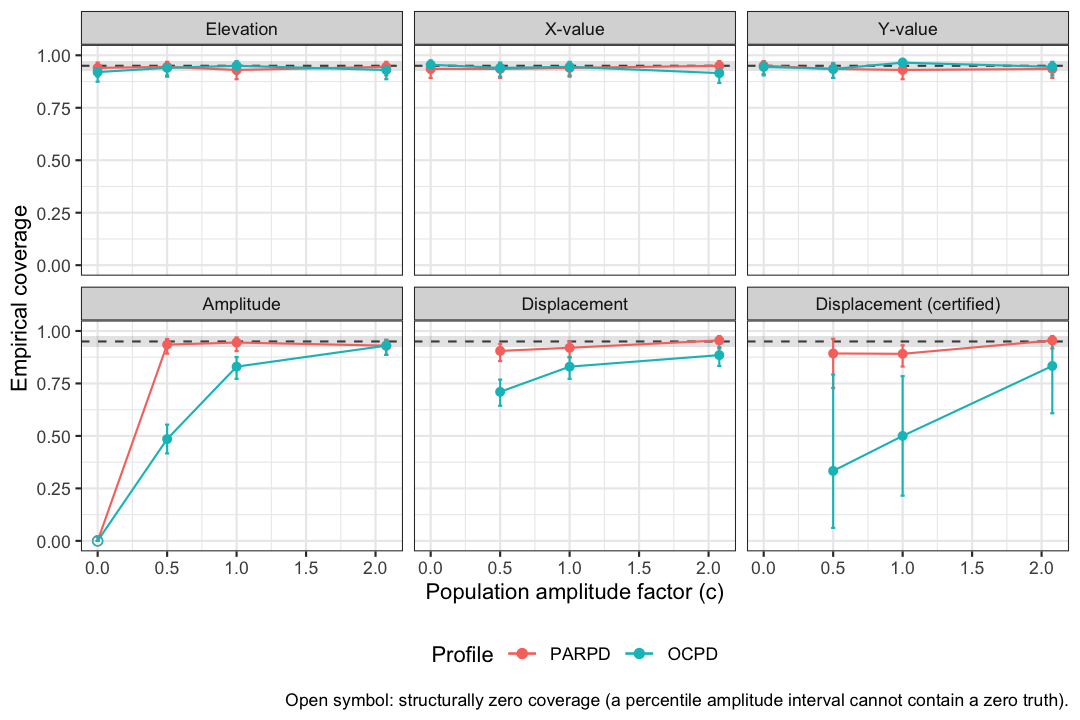

plot of chunk accuracy_plot

Two settings are worth knowing. First, structure = "observed" rebuilds the population from the pooled observed correlations instead of the CPM. If the two structures yield different verdicts, that disagreement is itself informative: structure uncertainty is material for your data. Second, the embedded CPM fit is returned as acc$cpm, for inspection with the tools from “Evaluating Circumplex Structure”.

The diagnostic itself was validated against Zimmermann and Wright’s published results. Configured to their transcribed simulation conditions, it reproduces their accuracy classifications. It gives coverage inside the Bradley band at conditions they found accurate. It gives the same one-sided under-coverage at conditions they found inaccurate.

4. When to trust SSM parameters

Putting “Evaluating Circumplex Structure” and this page together into a checklist:

Structure first. Fit cpm_fit() to your instrument in your sample. If the octant ordering fails or communalities are very low, stop, because SSM positions mean little.
Elevation is the robust parameter. It is essentially unbiased, and its intervals were accurate from $n \ge 50$ in every published and package-run condition. (On the correlation path, elevation is also the parameter that ipsatizing destroys. See “Structure Tests and Ipsatization”.)
Treat amplitude as optimistic. It cannot go below zero, so it overshoots when true differentiation is weak. Before interpreting a “marked” amplitude at modest $n$ , run ssm_ci_accuracy() and look at the sub-1 ladder rungs in its summary() or plot().
Only interpret displacement when amplitude is credible. When the amplitude CI lower bound sits less than 0.35 CI-widths above zero, the printed output notes that the displacement is not interpretable. The diagnostic tells you how reliable that certification is at your configuration.
Do not build claims on the fit parameter’s interval. Zimmermann and Wright found bootstrap $R^2$ intervals accurate only when population fit was mediocre. Near-perfect prototypicality cannot be bracketed from below. Report $R^2$ descriptively.
Remember what the diagnostic conditions on. It asks “would my CI procedure work in a population like my estimates”, under multivariate normality, with complete data. It is a strong check, not a certificate.

Wrap-up

Interval accuracy depends on the sample size, the instrument and how differentiated the profile really is, and ssm_ci_accuracy() measures it at your own configuration. The next page is “Structure Tests and Ipsatization”. It asks the exploratory version of the structure question and shows what ipsatizing removes from a profile.

References

Bradley, J. V. (1978). Robustness? British Journal of Mathematical and Statistical Psychology, 31(2), 144–152.
Zimmermann, J., & Wright, A. G. C. (2017). Beyond description in interpersonal construct validation: Methodological advances in the circumplex Structural Summary Approach. Assessment, 24(1), 3–23.