Latent Group Contrasts

library(circumplex)
data("jz2017")
scales <- c("PA", "BC", "DE", "FG", "HI", "JK", "LM", "NO")

Level: Advanced. Read “SEM-Based SSM Analysis” first.

1. Overview

This page continues “SEM-Based SSM Analysis”, which fits the latent profile of a measure with ssm_sem(). It teaches the second product of the latent SSM, the invariance-gated latent contrast between groups, and it places the method. The setup chunk loads jz2017 and names the eight scales, as the previous page did. Section 2, “Two questions about group differences”, separates the observed contrast from the latent one. Section 3, “Invariance-gated latent contrasts”, fits the invariance ladder and shows a comparison that the gate refuses. It then shows a contrast of two measures within one group, where no invariance gate applies. Section 4, “When to trust it: limitations”, lists the assumptions that the latent layer rests on. Section 5, “Relation to the literature”, places the method beside the published circumplex models. The Wrap-up restates when a latent contrast is computed and names the next page, and the References list the sources cited.

2. Two questions about group differences

When you have groups, there are two distinct estimands (quantities to be estimated), and circumplex keeps them separate on purpose.

Two estimands for a group difference

Question	Estimand	Tool	Confounds
Do the groups’ measured profiles differ?	Observed contrast	ssm_analyze(contrast = TRUE)	Structural difference, differential reliability, and non-invariance are combined.
Do the groups’ constructs differ, granted the instrument measures the same thing in both?	Latent contrast	ssm_sem(contrast = TRUE)	Disattenuated and conditional on measurement invariance; not computed when invariance fails.

Neither is more correct in the abstract. The observed contrast answers a question about scores and is always available. The latent contrast answers a question about constructs, but only if the instrument behaves the same way in both groups. When it does not, the honest answer is that the groups cannot be compared on the latent metric. That answer is not a number.

3. Invariance-gated latent contrasts

Before it computes a latent group contrast, ssm_sem() fits an invariance ladder: configural, then metric, then scalar. It tests each rung against the previous one with lavaan’s own nested-model test (the scaled difference test under the robust estimator). The latent measure-profile contrast requires metric invariance (equal saturations across groups). The latent mean contrast additionally requires scalar invariance. If the required rung is rejected, the contrast is not computed.

On real data this gate does its job. Comparing the NARPD profile across the Gender groups in jz2017 rejects metric invariance. So ssm_sem() returns each group’s separate profile and an explicit non-comparison verdict, rather than a contrast:

set.seed(12345)
by_gender <- ssm_sem(
  jz2017,
  scales = scales,
  angles = octants(),
  measures = "NARPD",
  grouping = "Gender",
  contrast = TRUE,
  boots = 300
)
by_gender
#> 
#> # Latent (SEM-based) SSM
#> 
#> Measurement model:    scaled fixed-angle circumplex
#> Global fit (N = 1166, robust): chisq(34) = 287.272, p < 0.001 
#>          CFI = 0.938, RMSEA = 0.123, SRMR = 0.06
#> 
#> Invariance ladder (gate: metric, alpha = 0.05):
#>        rung   chisq df   cfi rmsea dchisq ddf       p
#>  configural 287.272 34 0.938 0.123     NA  NA        
#>      metric 337.356 48 0.927 0.112 54.781  14 < 0.001
#> Verdict:    metric invariance rejected
#>   Test:     Δχ²(14) = 54.78, p < 0.0001, alpha = 0.05
#>   Result:   these groups cannot be compared on this instrument's latent
#>             metric
#>   Contrast: the requested latent contrast was not computed
#>   Profiles: the rows below are each group's separate (configural) latent
#>             profile
#>   Instead:  the observed-score contrast from ssm_analyze() answers a
#>             different question and remains available
#> 
#> # Profile [NARPD: Female]:
#> 
#>                Estimate   Lower CI   Upper CI
#> Elevation         0.198      0.141      0.252
#> X-Value          -0.023     -0.083      0.040
#> Y-Value           0.250      0.188      0.318
#> Amplitude         0.251      0.194      0.318
#> Displacement     95.206     81.443    110.519
#> Model Fit         0.966                      
#> 
#> 
#> # Profile [NARPD: Male]:
#> 
#>                Estimate   Lower CI   Upper CI
#> Elevation         0.313      0.243      0.376
#> X-Value           0.012     -0.046      0.076
#> Y-Value           0.199      0.146      0.250
#> Amplitude         0.199      0.147      0.257
#> Displacement     86.611     70.075    103.660
#> Model Fit         0.977

The invariance ladder is printed with the decision, and no contrast is rendered. The Verdict: line names the decision. The labeled lines under it give the nested test, what the decision means for comparing the groups, and what to use instead. ssm_plot_contrast() on this object would have nothing to draw. This is deliberate: there is no force = TRUE. If you have a principled partial-invariance model, fit it yourself and pass it to ssm_sem_parameters(). That function computes the contrast from whatever multi-group fit you supply, and it leaves the comparability claim to you.

The ladder table in the returned object also carries dcfi, the change in the comparative fit index (CFI) from the previous fitted rung. CFI compares the model’s fit with that of a baseline model in which the variables are uncorrelated, and values near 1 mean good fit. dcfi is Cheung and Rensvold’s (2002) secondary criterion. Its general rule rejects an invariance step when CFI falls by more than .01. It is reported, never gating. Comparability, the verdict, and the model that the estimates are taken from are decided by the nested test alone. The two criteria can disagree, and neither is a tiebreaker for the other. A change in CFI is insensitive to sample size, but the nested test is not. So in a large sample the nested test can reject a step whose CFI barely moves.

The direction of the ΔCFI rule is worth stating carefully, because the article gives it two ways. Its Table 5 reports critical values that are the 1% lower tails of the simulated null distributions. So a ΔCFI at or below one of them is the 1%-level evidence against invariance, which is the sense used here. The sentence stating the general rule on the article’s p. 251 reads the opposite way relative to that same table. This package follows the simulation.

Read the retain/reject label narrowly on the occasions it appears. Cheung and Rensvold simulated two groups, maximum likelihood (ML) estimation, and multivariate normal data. They examined Type I error only, not power, and robust CFI variants were not part of their study. ssm_sem() therefore prints the dcfi and cr columns and a short ΔCFI note only inside that envelope. That is a two-group fit estimated by ML whose CFI is the plain, non-robust one. Note that estimator = "ML" is necessary but not sufficient. missing = "fiml" also makes lavaan report a robust CFI, so a fit can be ML and still fall outside the envelope. The default estimator is "MLR". So the ladder above prints no dcfi column and no ΔCFI note. The values are still in by_gender$invariance$table$dcfi with no label, and by_gender$invariance$dcfi_scope records the fields that show which condition applies. The same withholding covers a non-ML estimator such as "GLS". Its CFI is plain-named, but its fit function is not the one that the criterion was simulated under. That is a deliberate refusal rather than a gap. Extending the cutoff to a robust index, another estimator, or three or more groups would take simulation work that nobody has done.

When invariance is not the obstacle, the contrast is computed. An example is a contrast of two measures within one group, where no cross-group invariance is at stake. That contrast behaves like the observed contrast (second measure minus first, displacement differences via the circular branch machinery):

set.seed(12345)
contrast <- ssm_sem(
  jz2017,
  scales = scales,
  angles = octants(),
  measures = c("NARPD", "ASPD"),
  contrast = TRUE,
  boots = 500
)
contrast
#> 
#> # Latent (SEM-based) SSM
#> 
#> Measurement model:    scaled fixed-angle circumplex
#> Global fit (N = 1166, robust): chisq(22) = 317.867, p < 0.001 
#>          CFI = 0.935, RMSEA = 0.114, SRMR = 0.068
#> 
#> # Profile [NARPD]:
#> 
#>                Estimate   Lower CI   Upper CI
#> Elevation         0.248      0.210      0.295
#> X-Value          -0.009     -0.052      0.032
#> Y-Value           0.231      0.191      0.272
#> Amplitude         0.231      0.193      0.272
#> Displacement     92.119     82.715    103.513
#> Model Fit         0.974                      
#> 
#> 
#> # Profile [ASPD]:
#> 
#>                Estimate   Lower CI   Upper CI
#> Elevation         0.161      0.115      0.207
#> X-Value          -0.043     -0.092     -0.002
#> Y-Value           0.250      0.208      0.295
#> Amplitude         0.254      0.216      0.298
#> Displacement     99.732     90.351    111.188
#> Model Fit         0.978                      
#> 
#> 
#> # Contrast [ASPD - NARPD]:
#> 
#>                  Estimate   Lower CI   Upper CI
#> Δ Elevation        -0.087     -0.138     -0.044
#> Δ X-Value          -0.034     -0.084      0.019
#> Δ Y-Value           0.019     -0.028      0.066
#> Δ Amplitude         0.022     -0.025      0.066
#> Δ Displacement      7.613     -6.113     19.993
#> Δ Model Fit         0.003

ssm_plot_contrast(contrast)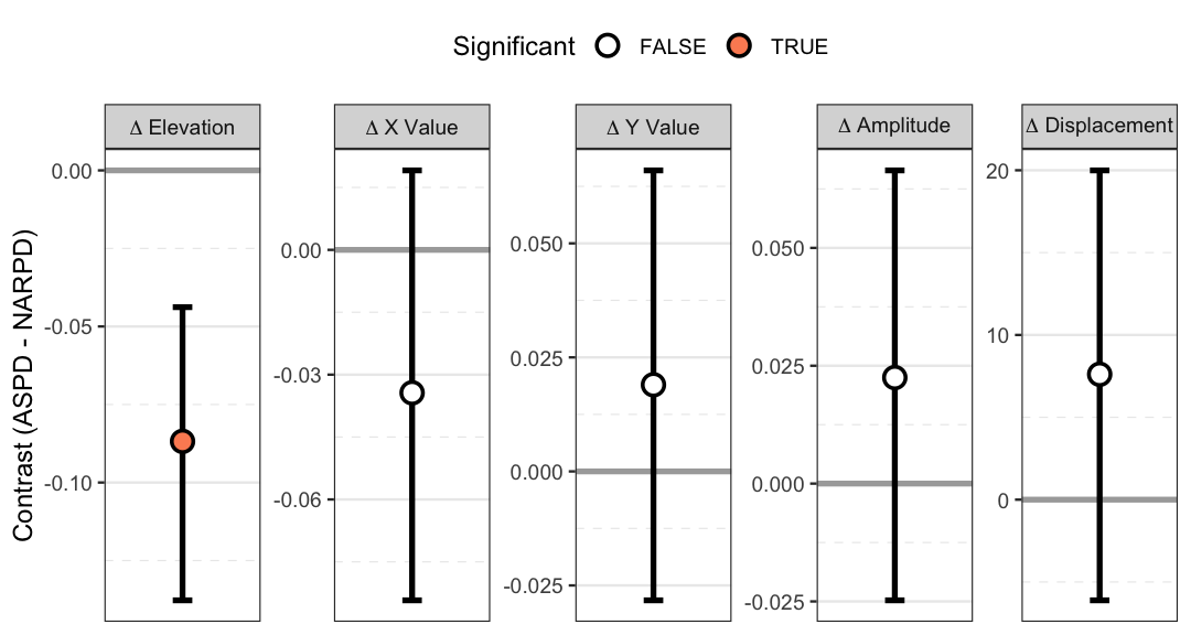

The contrast block reports the difference in each SSM parameter with its confidence interval. As with the observed contrast, an elevation or amplitude difference whose interval excludes zero is a difference in that parameter. The displacement difference is reported on the estimate’s angular branch. So its interval endpoints can legitimately fall outside ±180° near the boundary, while still containing the estimate.

4. When to trust it: limitations

The latent layer buys disattenuation at the price of a set of assumptions. The documentation states them, and the vignette should too.

• Model-conditional. Every latent quantity is conditional on the fixed-angle model being adequate. Read the global fit first. Wendt et al.
  2019. give a real-data benchmark. They reported RMSEA (a misfit index, where lower is better) between .075 and .111 across four large samples. Their model was the fixed-loading circumplex confirmatory factor analysis (CFA), and these values show a real but imperfect approximation. Their model targets the octants’ own latent structure, not an external measure’s profile. So the number is a benchmark, not a like-for-like comparison. The example fits here are of the same order (RMSEA around .12). They should likewise be read as approximations, not exact structure.
• Fixed angles are theoretical. Departures from the theoretical geometry load into misfit, not into the angles. Use cpm_fit() to examine geometry.
• The scaled tier assumes latent-plane stationarity and does not test it. That tier fixes the plane factors isotropic and orthogonal, so anisotropic latent dispersion surfaces only as global misfit. The strict tier frees the factor variances and covariances.
• The scaled tier assumes the general factor is orthogonal to the plane. A true general-factor lean surfaces as misfit under the scaled tier. Use the strict tier to model it.
• Displacement and fit have the disattenuated meanings of Section 6 of “SEM-Based SSM Analysis”, not the naive “angle in latent space” and “cosine-ness” readings.
• Disattenuated correlations can be large. Removing attenuation moves correlations toward ±1. Values at or beyond 1 signal misspecification and are refused rather than summarized.
• Invariance gating is a modeling decision with a default test, not an oracle. The observed contrast remains available and answers its own question. The secondary dcfi criterion gates nothing. It prints beside the nested test only for a two-group fit estimated by ML with a plain CFI. Even then it prints only when a rung has a dcfi value. Its .01 cutoff is validated only for two-group, ML, multivariate-normal fits, for Type I error only. The package withholds the verdict everywhere else rather than extrapolating it.

5. Relation to the literature

The nearest published models are the confirmatory factor analyses of the interpersonal circumplex itself. Wendt et al. (2019) fit a three-factor circumplex CFA with fixed unit-cosine plane loadings, which is the shape of this package’s strict tier. They fit it across four large samples. They found the fully dimensional model competitive with categorical (types of people) and hybrid (types and dimensions together) alternatives. Their estimand, though, is the latent structure of the octant scales and persons’ factor scores, not an external measure’s disattenuated profile. Their model is context for the strict tier, not a validation target for the SSM estimand.

At the level of a single disattenuated correlation, Moss (2026) showed the following. Treating reliability as a known constant collapses interval coverage (to roughly .35 in one scenario). Propagating reliability uncertainty instead restores nominal coverage. That is exactly the logic behind fitting the model and propagating its full covariance, rather than plugging in reliability point estimates. One estimand caveat applies. Moss’s disattenuated correlation corrects both variables for unreliability. The latent SSM here corrects only the scale side, and the external measure remains an observed variable. So the two are relatives, not the same quantity.

Finally, the two model families in this package meet at a single point. At that point the general factor is orthogonal to the plane, the saturations are equal, and the angles are equally spaced. At that point, the fixed-loading circumplex CFA coincides with the one-harmonic, equal-communality version of Browne’s (1992) circumplex model that cpm_fit() estimates. The SEM-based SSM sits on the fixed-angle side of that boundary. To cross to freely estimated angles, use cpm_fit().

Wrap-up

ssm_sem() computes a latent group contrast only when the invariance ladder supports it. When the ladder does not, it returns each group’s separate profile with a verdict. A contrast of two measures within one group needs no invariance gate. The next page to read is “Axes Reliability”, which asks how reliably an instrument measures its two axes.

References

• Browne, M. W. (1992). Circumplex models for correlation matrices. Psychometrika, 57(4), 469–497.

• Cheung, G. W., & Rensvold, R. B. (2002). Evaluating goodness-of-fit indexes for testing measurement invariance. Structural Equation Modeling, 9(2), 233–255.

• Moss, J. (2026). Inference for disattenuated correlations. Applied Psychological Measurement. Advance online publication. https://doi.org/10.1177/01466216261440511

• Wendt, L. P., Wright, A. G. C., Pilkonis, P. A., Nolte, T., Fonagy, P., Montague, P. R., Benecke, C., Krieger, T., & Zimmermann, J. (2019). The latent structure of interpersonal problems: Validity of dimensional, categorical, and hybrid models. Journal of Abnormal Psychology, 128(8), 823–839.