Trajectory of SSM parameters from a fitted growth model

Turn the fixed effects of the joint growth model that ssm_growth_formula() builds into a table of Structural Summary Method parameters at each time point, with intervals and the displacement certification. Two input shapes are accepted. The frequentist shape is coef and vcov, the fixed effects and their covariance from a glmmTMB or nlme fit. The function draws n_draws coefficient vectors from the multivariate normal distribution they define, the same large-sample step the package's Monte Carlo method takes. The Bayesian shape is draws, a matrix of posterior coefficient draws such as as.matrix(fit) from brms, used as given. Under either shape, each draw's e, x and y at time t are its intercept plus t times its slope, and the draws at each time go through ssm_draws() with type = "parameters".

Usage

ssm_trajectory(
  coef,
  vcov,
  times,
  draws = NULL,
  time = "wave",
  interval = 0.95,
  n_draws = 4000,
  contrast = NULL
)

# S3 method for class 'circumplex_ssm_trajectory'
print(x, digits = 2, ...)

# S3 method for class 'circumplex_ssm_trajectory'
rbind(..., deparse.level = 1, make.row.names = TRUE, stringsAsFactors = FALSE)

Arguments

coef: The fixed effects: a named numeric vector. Required with vcov, and absent with draws.
vcov: The covariance matrix of coef: a symmetric numeric matrix with one row and column per element of coef, its dimnames equal to names(coef) when present. Required with coef, and absent with draws.
times: Required. A numeric vector of the time values at which to evaluate the trajectory, one output row each.
draws: Optional. A numeric matrix of coefficient draws, one row per draw and one named column per coefficient, in place of coef and vcov. When given, n_draws is ignored.
time: Optional. The name of the time column in the output, and the suffix of the slope coefficients (default "wave"), the same time given to ssm_growth_data() and ssm_growth_formula().
interval: Optional. A single number between 0 and 1 giving the level of the intervals (default = 0.95).
n_draws: Optional. The number of coefficient vectors to draw from coef and vcov (default = 4000).
contrast: Optional. NULL (default) for the default contrast, or a function of one time value returning a 3 by p numeric matrix whose rows are e, x and y and whose columns follow the order of coef or of the columns of draws.
x: An object of class "circumplex_ssm_trajectory".
digits: The number of decimal places to print (default = 2).
...: For print(), ignored (S3 consistency). For rbind(), the trajectory tables to stack.
deparse.level, make.row.names, stringsAsFactors: For rbind(), passed to rbind.data.frame().

Value

A data frame of class "circumplex_ssm_trajectory" with attribute time naming its time column and attribute input recording the input shape, "coef_vcov" or "draws", one row per value of times. Its columns are <time>; e_est, e_lci, e_uci, and the same three for x, y, a and d; and certified. The estimates and bounds are those ssm_draws() reports: medians and equal-tailed interval bounds for e, x, y and a, and the circular mean with circular quantile bounds in degrees for d. A d interval that straddles 0/360 degrees has d_lci > d_uci. certified is the displacement certification at that time, and at an uncertified time the d interval is not interpretable. Printing shows the table rounded, marks each uncertified row, and ends with the caution for the input shape: the small-sample caution under coef and vcov, and under draws that the intervals summarize the draws as given. A subset that drops the attribute, or an rbind() of trajectory tables of different shapes, prints a caution that says the shape is not recorded. ssm_plot_trajectory() plots the object with no time argument.

Details

The default contrast reads six coefficient names: dve, dvx, dvy and dve:<time>, dvx:<time>, dvy:<time>, where <time> is the time argument. Those are the names the model from ssm_growth_formula() gives its fixed effects on the long table ssm_growth_data() builds. A b_ prefix on the column names of draws is dropped, and other columns, such as brms's sd_, cor_ and lp__ columns, are ignored. A missing name is an error. A contrast function replaces the default for a model with other terms, such as a quadratic time term; it must return, for one time value, the 3 by p matrix that maps the p coefficients to e, x and y at that time, in coefficient order.

The displacement interval at a time point is wrong when x(t) and y(t) are treated as independent, which is what fitting the coordinates in separate models does. So the coef and vcov shape refuses a vcov whose implied covariance between x(t) and y(t) is exactly zero at every time in times, unless vcov is zero everywhere. The check reads only the given times, so with a single time it sees only the covariance terms that time reaches. A draws matrix is not checked for a joint fit. The intervals from a REML fit's coef and vcov condition on its estimated variance components and are too narrow at small samples; the "Growth Models on SSM Parameters" vignette, Section 7, states what the package's coverage oracle measured and that no shipped correction exists. Intervals from draws summarize those draws as given.

Examples

# Fixed effects and covariance in the shape a joint fit returns
coef <- c(
  dve = 0.52, dvx = 0.61, dvy = -0.10,
  "dve:wave" = 0.00, "dvx:wave" = 0.00, "dvy:wave" = 0.065
)
vcov <- diag(c(7e-4, 3e-4, 3e-4, 5e-5, 2e-5, 2e-5))
vcov[2, 3] <- vcov[3, 2] <- 4e-5
dimnames(vcov) <- list(names(coef), names(coef))
set.seed(1)
trajectory <- ssm_trajectory(coef, vcov, times = 0:4)
trajectory
#> 
#> # SSM Trajectory:
#> 
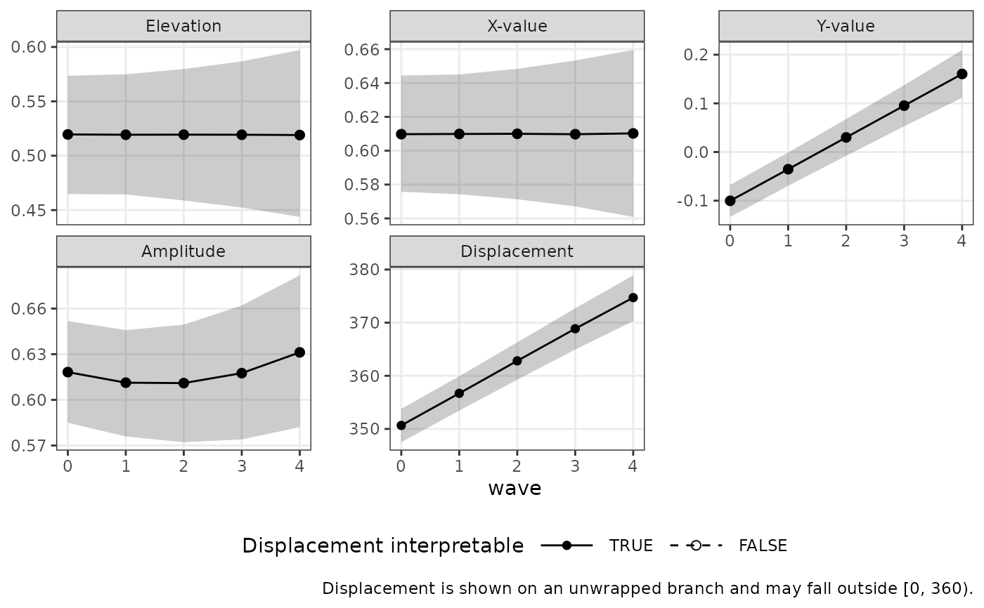
#>  wave e_est e_lci e_uci x_est x_lci x_uci y_est y_lci y_uci a_est a_lci a_uci
#>     0  0.52  0.46  0.57  0.61  0.58  0.64 -0.10 -0.13 -0.07  0.62  0.58  0.65
#>     1  0.52  0.46  0.57  0.61  0.57  0.65 -0.04 -0.07  0.00  0.61  0.58  0.65
#>     2  0.52  0.46  0.58  0.61  0.57  0.65  0.03 -0.01  0.07  0.61  0.57  0.65
#>     3  0.52  0.45  0.59  0.61  0.57  0.65  0.10  0.05  0.14  0.62  0.57  0.66
#>     4  0.52  0.44  0.60  0.61  0.56  0.66  0.16  0.11  0.21  0.63  0.58  0.68
#>   d_est  d_lci  d_uci
#>  350.66 347.50 353.78
#>  356.70 353.44 359.92
#>    2.81 359.25   6.30
#>    8.86   4.94  12.71
#>   14.72  10.31  18.92
#>   Caution: intervals from a fitted model's fixed-effect covariance condition on
#>   its estimated variance components, and are too narrow at small samples. See
#>   vignette("growth-ssm-analysis"), Section 7.
#> 
ssm_plot_trajectory(trajectory)


# The same from a matrix of coefficient draws, here drawn by hand; a brms
# fit gives one as `as.matrix(fit)`
set.seed(1)
draws <- matrix(rnorm(500 * 6), nrow = 500) %*% chol(vcov)
draws <- sweep(draws, 2, coef, "+")
colnames(draws) <- names(coef)
ssm_trajectory(times = 0:4, draws = draws)
#> 
#> # SSM Trajectory:
#> 
#>  wave e_est e_lci e_uci x_est x_lci x_uci y_est y_lci y_uci a_est a_lci a_uci
#>     0  0.52  0.47  0.57  0.61  0.57  0.64 -0.10 -0.13 -0.06  0.62  0.58  0.65
#>     1  0.52  0.47  0.57  0.61  0.57  0.65 -0.04 -0.07  0.00  0.61  0.57  0.65
#>     2  0.52  0.46  0.58  0.61  0.57  0.65  0.03 -0.01  0.07  0.61  0.57  0.65
#>     3  0.52  0.45  0.59  0.61  0.57  0.65  0.09  0.05  0.14  0.62  0.57  0.66
#>     4  0.52  0.44  0.60  0.61  0.56  0.66  0.16  0.11  0.21  0.63  0.58  0.68
#>   d_est  d_lci  d_uci
#>  350.66 347.72 353.89
#>  356.70 353.46   0.11
#>    2.82 359.32   6.68
#>    8.87   4.99  13.00
#>   14.72  10.27  19.40
#>   Caution: these intervals summarize the supplied draws as given. Their coverage
#>   depends on how the draws were produced, and the joint fit was not checked. See
#>   vignette("growth-ssm-analysis"), Sections 7 and 10.
#>