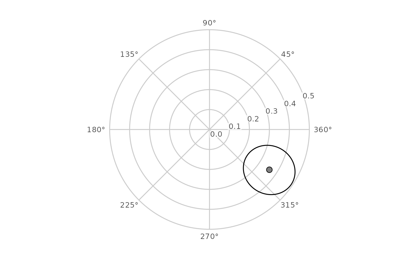
Draw a joint confidence ellipse for SSM coordinates in circumplex space

A ggplot2 layer that draws, for each profile, the ellipse of a bivariate normal region on the Cartesian (x, y) coordinates of the Structural Summary Method, on a circumplex canvas built with coord_circumplex() (for example the canvas from ggcircumplex()). Each row supplies the centre (x0, y0) and the three elements of a 2 by 2 covariance matrix; the layer computes the ellipse's outline in Cartesian space, converts each vertex to a displacement and an amplitude, and hands those to the coordinate system, which owns the polar transform.

Usage

geom_ssm_ellipse(
  mapping = NULL,
  data = NULL,
  stat = "identity",
  position = "identity",
  ...,
  level = 0.95,
  n = 100,
  na.rm = TRUE,
  show.legend = NA,
  inherit.aes = TRUE
)

Arguments

mapping, data, stat, position, show.legend, inherit.aes, ...: Standard ggplot2 layer arguments. mapping must supply the x0, y0, var_x, var_y, and cov_xy aesthetics: the centre and the variances of x and y and their covariance, all in the score metric of the Cartesian coordinates.
level: A single number strictly between 0 and 1: the confidence level of the region (default 0.95).
n: The number of vertices on each outline (default 100), a single whole number of at least 3; the path returns to its first vertex.
na.rm: If FALSE, warn (with the dropped-row count) before removing rows with a non-finite centre or covariance element; if TRUE (the default) remove them silently. A covariance that is not positive definite is an error, not a missing value.

Value

A ggplot2 layer.

Details

The outline is the contour (v - c)' S^-1 (v - c) = qchisq(level, 2), where c is the centre and S the covariance: under a bivariate normal approximation to the distribution of (x, y), sampling or posterior, it encloses the joint region at confidence level. ssm_ellipse_data() computes the five columns from an ssm_draws() object. The ellipse is a statement about the Cartesian pair, not about amplitude and displacement separately; the wedge geom_ssm_arc() draws is the pair of marginal intervals on those two parameters, and the two regions need not coincide.

Vertices are unwrapped along the outline so that an ellipse straddling the 0/360 seam is drawn across it, and an ellipse whose inscribed polygon contains the origin winds once round the centre of the canvas. Unwrapped displacements may therefore fall outside [0, 360). Each retained input row is one outline: the layer sets the group aesthetic to one value per retained row, replacing any group the mapping supplies.

Examples

set.seed(1)
draws <- cbind(rnorm(500, 0.4, 0.1), rnorm(500, 0.3, 0.05),
               rnorm(500, -0.2, 0.05))
res <- ssm_draws(draws, type = "parameters")
ggcircumplex(octants(), amax = 0.5) +
  geom_ssm_ellipse(
    data = ssm_ellipse_data(res),
    mapping = ggplot2::aes(
      x0 = x0, y0 = y0, var_x = var_x, var_y = var_y, cov_xy = cov_xy
    )
  ) +
  geom_ssm_point(
    data = res$results,
    mapping = ggplot2::aes(amplitude = a_est, displacement = d_est)
  )