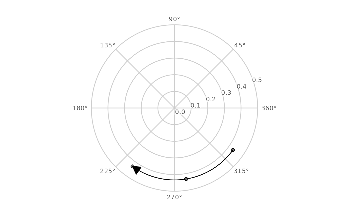
Draw a profile's movement across occasions in circumplex space

A ggplot2 layer that connects a profile's successive positions on a circumplex canvas built with coord_circumplex() (for example the canvas from ggcircumplex()), so change in amplitude and displacement reads as movement through circumplex space. Each segment is curved along the polar geodesic by the coordinate system, which owns the transform; the layer owns the ordering, the 0/360 seam handling, and the optional arrowheads.

Usage

geom_ssm_path(
  mapping = NULL,
  data = NULL,
  stat = "identity",
  position = "identity",
  ...,
  arrow = NULL,
  na.rm = TRUE,
  show.legend = NA,
  inherit.aes = TRUE
)

Arguments

mapping, data, stat, position, show.legend, inherit.aes, ...

Standard ggplot2 layer arguments. mapping must supply the amplitude and displacement aesthetics.

arrow

An arrow specification produced by ggplot2::arrow(), or NULL (the default) for a path drawn without arrowheads. Arrowheads mark the direction of time along the path.

na.rm

If FALSE, warn when occasions with no location are removed from the ends of a path; if TRUE (the default) remove them silently. Occasions with no location in the middle of a path break it either way.

Value

A ggplot2 layer.

Details

Points are connected in the order the rows appear in the data, exactly as ggplot2::geom_path() does, and the group aesthetic separates one series from another. Sort the data into time order before plotting: an occasion label sorted as text puts T10 before T2, which silently reverses time. ssm_plot_circle(path = TRUE) does this sorting for you, taking the order from the object's own occasion list.

Consecutive occasions are joined the short way around the circle. The displacements of each group are unwrapped onto a continuous branch before the coordinate system sees them, so a step from 350 to 10 degrees is drawn as the 20 degree arc across the pole rather than a 340 degree sweep the long way round. Unwrapped values may therefore fall outside [0, 360). This assumes the profile rotates less than a half-turn between consecutive occasions at which its displacement is defined; no data can verify that, so widely spaced occasions should be read with it in mind.

An occasion with no defined location – a flat or zero-amplitude profile, whose displacement is undefined – breaks the path rather than being interpolated through, and the segment after the gap is still drawn on the correct branch. Non-finite amplitudes and displacements are treated the same way, since an infinite angle names no position on the circle.

See also

Other circumplex layers: coord_circumplex(), geom_ssm_arc(), geom_ssm_point(), ggcircumplex(), scale_x_circumplex(), theme_circumplex()

Examples

data("jz2017")
scales <- c("PA", "BC", "DE", "FG", "HI", "JK", "LM", "NO")
# Three occasions that actually move: shifting the octant scores by one
# position rotates the fitted profile by 45 degrees per occasion.
waves <- lapply(1:3, function(k) {
  idx <- ((seq_along(scales) - 1 + (k - 1)) %% length(scales)) + 1
  d <- jz2017[, scales[idx]]
  names(d) <- scales
  d$id <- seq_len(nrow(d))
  d$occasion <- paste0("T", k)
  d
})
res <- ssm_analyze_long(do.call(rbind, waves),
  scales = scales, id = "id", occasion = "occasion"
)
ggcircumplex(octants(), amax = 0.5) +
  geom_ssm_point(
    data = res$results,
    mapping = ggplot2::aes(amplitude = a_est, displacement = d_est),
    size = 2
  ) +
  geom_ssm_path(
    data = res$results,
    mapping = ggplot2::aes(amplitude = a_est, displacement = d_est),
    arrow = ggplot2::arrow(
      length = ggplot2::unit(0.18, "inches"), type = "closed"
    )
  )